Influenza Project - TidyModels Analysis (Part 1)

Introduction

This exercise focuses on applying the base TidyModels framework to the influenza data, and most of the code comes from the TidyModels’ “Build a Model” Tutorial.

The raw data for this exercise comes from the following citation: McKay, Brian et al. (2020), Virulence-mediated infectiousness and activity trade-offs and their impact on transmission potential of patients infected with influenza, Dryad, Dataset, https://doi.org/10.5061/dryad.51c59zw4v.

The processed data was produced on the Data Processing page.

Within this analysis, the following definitions exist:

Main predictor of interest = Runny Nose
Continuous outcome of interest = Body Temperature
Categorical outcome of interest = Nausea
Whichever outcome is not currently fitted will be considered a predictor of interest
All variables are included (even when there are multiple variables for the same symptom)

The overall steps of this exercise are as follows:

Load the processed data
Fit a linear model to the continuous outcome using only the main predictor of interest
Fit another linear model to the continuous outcome using all predictors of interest
Compare model results for models created in steps (2) and (3)
Fit a logistic model to the categorical outcome using only the main predictor of interest
Fit another logistic model to the categorical outcome using all predictors of interest
Compare model results for models created in steps (5) and (6)

Required Packages

The following R packages are required for this exercise:

here: for path setting
tidyverse: for all packages in the Tidyverse (ggplot2, dyplr, tidyr, readr, purr, tibble, stringr, forcats)
summarytools: for overall dataframe summary
ggplot2: for plotting data
tidymodels: for all packages in the TidyModels suite
broom.mixed: for converting bayesian models to tidy tibbles
broom: for model organization / clarity
dotwhisker: for visualizing regression results
gtsummary: for converting regression results to table
modelsummary: for comparing results of models
flextable: for exporting tables

Load Processed Data

Load the data created on the Data Processing page.

# path to data
# note the use of the here() package and not absolute paths
data_location <- here::here("data","flu","processeddata.rds")

# load data using the "ReadRDS" function in base R.
mydata <- base::readRDS(data_location)

Data Summary

For a more robust exploration, refer to the Exploratory Data Analysis page. However, for reference, we can look at the dataframe summary using the skimr package.

#summary of data using skimr package
skimr::skim(mydata)

Data summary
Name	mydata
Number of rows	730
Number of columns	32
_______________________
Column type frequency:
factor	31
numeric	1
________________________
Group variables	None

Variable type: factor

skim_variable	complete_rate	ordered	n_unique	top_counts
SwollenLymphNodes	1	FALSE	2	No: 418, Yes: 312
ChestCongestion	1	FALSE	2	Yes: 407, No: 323
ChillsSweats	1	FALSE	2	Yes: 600, No: 130
NasalCongestion	1	FALSE	2	Yes: 563, No: 167
CoughYN	1	FALSE	2	Yes: 655, No: 75
Sneeze	1	FALSE	2	Yes: 391, No: 339
Fatigue	1	FALSE	2	Yes: 666, No: 64
SubjectiveFever	1	FALSE	2	Yes: 500, No: 230
Headache	1	FALSE	2	Yes: 615, No: 115
Weakness	1	FALSE	4	Mod: 338, Mil: 223, Sev: 120, Non: 49
WeaknessYN	1	FALSE	2	Yes: 681, No: 49
CoughIntensity	1	FALSE	4	Mod: 357, Sev: 172, Mil: 154, Non: 47
CoughYN2	1	FALSE	2	Yes: 683, No: 47
Myalgia	1	FALSE	4	Mod: 325, Mil: 213, Sev: 113, Non: 79
MyalgiaYN	1	FALSE	2	Yes: 651, No: 79
RunnyNose	1	FALSE	2	Yes: 519, No: 211
AbPain	1	FALSE	2	No: 639, Yes: 91
ChestPain	1	FALSE	2	No: 497, Yes: 233
Diarrhea	1	FALSE	2	No: 631, Yes: 99
EyePn	1	FALSE	2	No: 617, Yes: 113
Insomnia	1	FALSE	2	Yes: 415, No: 315
ItchyEye	1	FALSE	2	No: 551, Yes: 179
Nausea	1	FALSE	2	No: 475, Yes: 255
EarPn	1	FALSE	2	No: 568, Yes: 162
Hearing	1	FALSE	2	No: 700, Yes: 30
Pharyngitis	1	FALSE	2	Yes: 611, No: 119
Breathless	1	FALSE	2	No: 436, Yes: 294
ToothPn	1	FALSE	2	No: 565, Yes: 165
Vision	1	FALSE	2	No: 711, Yes: 19
Vomit	1	FALSE	2	No: 652, Yes: 78
Wheeze	1	FALSE	2	No: 510, Yes: 220

Variable type: numeric

skim_variable	n_missing	complete_rate	mean	sd	p0	p25	p50	p75	p100	hist
BodyTemp	0	1	98.94	1.2	97.2	98.2	98.5	99.3	103.1	▇▇▂▁▁

Linear Model for Body Temperature with Runny Nose

The first linear model to create is a simple one using the continuous outcome of interest (BodyTemp) and main predictor of interest (RunnyNose). Using the parsnip package, specify the functional form of the model (linear regression) and method for fitting the model, aka engine (“lm”).

#save the model object as lm_mod
lm_mod <-
  parsnip::linear_reg() %>%
  parsnip::set_engine("lm")

Now estimate the model using the fit function and summarize the linear model.

lm_fit1 <- lm_mod %>%
              fit(BodyTemp ~ RunnyNose, data = mydata)

#summarize linear model
lm_fit1_summary <- broom.mixed::tidy(lm_fit1)
lm_fit1_summary

## # A tibble: 2 x 5
##   term         estimate std.error statistic p.value
##   <chr>           <dbl>     <dbl>     <dbl>   <dbl>
## 1 (Intercept)    99.1      0.0819   1210.   0      
## 2 RunnyNoseYes   -0.293    0.0971     -3.01 0.00268

The intercept estimate (no runny nose) is 99.1F, which would make these patients febrile. We can interpret the slope estimate as: Patients with a runny nose on average have a 0.293F lower body temperature than patients without a runny nose.

Next, we can create a box and whisker plot for lm_fit1 output.

lm_fit1_bp <- broom.mixed::tidy(lm_fit1) %>%
                dotwhisker::dwplot(dot_args = list(size = 2, color = "blue"),
                                   whisker_args = list(color = "blue"),
                                   vline = geom_vline(xintercept = 0, colour = "grey50", linetype = 2))
lm_fit1_bp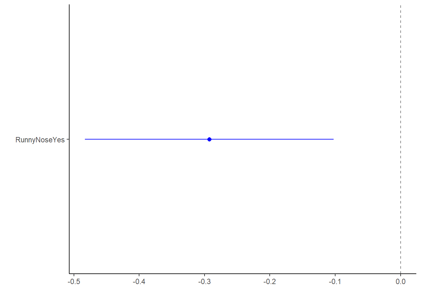

This shows us the estimate is significant (i.e. doesn’t cross the null hypothesis), and runny nose is a protective factor against increased body temperature.

Last, we can use the glance function to examine goodness of fit measures.

lm_fit1_gf <- modelsummary::glance(lm_fit1)
lm_fit1_gf

## # A tibble: 1 x 12
##   r.squared adj.r.squared sigma statistic p.value    df logLik   AIC   BIC
##       <dbl>         <dbl> <dbl>     <dbl>   <dbl> <dbl>  <dbl> <dbl> <dbl>
## 1    0.0123        0.0110  1.19      9.08 0.00268     1 -1162. 2329. 2343.
## # ... with 3 more variables: deviance <dbl>, df.residual <int>, nobs <int>

This model has an extremely low R^2, high AIC, BIC.

Linear Model for Body Temperature with All Predictors

The second linear model to create includes all variables in the dataset as predictors with the main outcome of interest as BodyTemp. We can use the same lm_mod function, so no need to respecify.

#create model including all predictors (defined using the . instead of specifying all variable names)
#doesn't include interaction terms
lm_fit2 <- lm_mod %>%
              fit(BodyTemp ~ ., data = mydata)

Now we can summarize the full linear model

#add print function to show all rows
lm_fit2_summary <- print(broom.mixed::tidy(lm_fit2), n = 38)

## # A tibble: 38 x 5
##    term                   estimate std.error statistic    p.value
##    <chr>                     <dbl>     <dbl>     <dbl>      <dbl>
##  1 (Intercept)            97.9        0.304   322.      0        
##  2 SwollenLymphNodesYes   -0.165      0.0920   -1.80    0.0727   
##  3 ChestCongestionYes      0.0873     0.0975    0.895   0.371    
##  4 ChillsSweatsYes         0.201      0.127     1.58    0.114    
##  5 NasalCongestionYes     -0.216      0.114    -1.90    0.0584   
##  6 CoughYNYes              0.314      0.241     1.30    0.193    
##  7 SneezeYes              -0.362      0.0983   -3.68    0.000249 
##  8 FatigueYes              0.265      0.161     1.65    0.0996   
##  9 SubjectiveFeverYes      0.437      0.103     4.22    0.0000271
## 10 HeadacheYes             0.0115     0.125     0.0913  0.927    
## 11 WeaknessMild            0.0182     0.189     0.0964  0.923    
## 12 WeaknessModerate        0.0989     0.198     0.500   0.617    
## 13 WeaknessSevere          0.373      0.231     1.62    0.106    
## 14 WeaknessYNYes          NA         NA        NA      NA        
## 15 CoughIntensityMild      0.0849     0.280     0.303   0.762    
## 16 CoughIntensityModerate -0.0614     0.302    -0.203   0.839    
## 17 CoughIntensitySevere   -0.0373     0.314    -0.119   0.906    
## 18 CoughYN2Yes            NA         NA        NA      NA        
## 19 MyalgiaMild             0.164      0.160     1.02    0.307    
## 20 MyalgiaModerate        -0.0241     0.168    -0.143   0.886    
## 21 MyalgiaSevere          -0.129      0.208    -0.622   0.534    
## 22 MyalgiaYNYes           NA         NA        NA      NA        
## 23 RunnyNoseYes           -0.0805     0.109    -0.742   0.459    
## 24 AbPainYes               0.0316     0.140     0.225   0.822    
## 25 ChestPainYes            0.105      0.107     0.982   0.326    
## 26 DiarrheaYes            -0.157      0.130    -1.21    0.227    
## 27 EyePnYes                0.132      0.130     1.01    0.311    
## 28 InsomniaYes            -0.00682    0.0908   -0.0752  0.940    
## 29 ItchyEyeYes            -0.00802    0.110    -0.0727  0.942    
## 30 NauseaYes              -0.0341     0.102    -0.334   0.739    
## 31 EarPnYes                0.0938     0.114     0.824   0.410    
## 32 HearingYes              0.232      0.222     1.05    0.296    
## 33 PharyngitisYes          0.318      0.121     2.62    0.00906  
## 34 BreathlessYes           0.0905     0.0998    0.907   0.365    
## 35 ToothPnYes             -0.0229     0.114    -0.201   0.841    
## 36 VisionYes              -0.275      0.278    -0.989   0.323    
## 37 VomitYes                0.165      0.151     1.09    0.275    
## 38 WheezeYes              -0.0467     0.107    -0.436   0.663

lm_fit2_summary

## # A tibble: 38 x 5
##    term                 estimate std.error statistic   p.value
##    <chr>                   <dbl>     <dbl>     <dbl>     <dbl>
##  1 (Intercept)           97.9       0.304   322.     0        
##  2 SwollenLymphNodesYes  -0.165     0.0920   -1.80   0.0727   
##  3 ChestCongestionYes     0.0873    0.0975    0.895  0.371    
##  4 ChillsSweatsYes        0.201     0.127     1.58   0.114    
##  5 NasalCongestionYes    -0.216     0.114    -1.90   0.0584   
##  6 CoughYNYes             0.314     0.241     1.30   0.193    
##  7 SneezeYes             -0.362     0.0983   -3.68   0.000249 
##  8 FatigueYes             0.265     0.161     1.65   0.0996   
##  9 SubjectiveFeverYes     0.437     0.103     4.22   0.0000271
## 10 HeadacheYes            0.0115    0.125     0.0913 0.927    
## # ... with 28 more rows

#the NA lines are where all patients are reporting the symptom (so no comparison possibility)

#export results into a table using the gtsummary package
gtsummary::tbl_regression(lm_fit2)

## Extracting {parsnip} model fit with `tbl_regression(x = x$fit, ...)`

Characteristic	Beta	95% CI¹	p-value
SwollenLymphNodes
No	—	—
Yes	-0.17	-0.35, 0.02	0.073
ChestCongestion
No	—	—
Yes	0.09	-0.10, 0.28	0.4
ChillsSweats
No	—	—
Yes	0.20	-0.05, 0.45	0.11
NasalCongestion
No	—	—
Yes	-0.22	-0.44, 0.01	0.058
CoughYN
No	—	—
Yes	0.31	-0.16, 0.79	0.2
Sneeze
No	—	—
Yes	-0.36	-0.55, -0.17	<0.001
Fatigue
No	—	—
Yes	0.26	-0.05, 0.58	0.10
SubjectiveFever
No	—	—
Yes	0.44	0.23, 0.64	<0.001
Headache
No	—	—
Yes	0.01	-0.23, 0.26	>0.9
Weakness
None	—	—
Mild	0.02	-0.35, 0.39	>0.9
Moderate	0.10	-0.29, 0.49	0.6
Severe	0.37	-0.08, 0.83	0.11
WeaknessYN
No	—	—
Yes
CoughIntensity
None	—	—
Mild	0.08	-0.46, 0.63	0.8
Moderate	-0.06	-0.65, 0.53	0.8
Severe	-0.04	-0.65, 0.58	>0.9
CoughYN2
No	—	—
Yes
Myalgia
None	—	—
Mild	0.16	-0.15, 0.48	0.3
Moderate	-0.02	-0.35, 0.31	0.9
Severe	-0.13	-0.54, 0.28	0.5
MyalgiaYN
No	—	—
Yes
RunnyNose
No	—	—
Yes	-0.08	-0.29, 0.13	0.5
AbPain
No	—	—
Yes	0.03	-0.24, 0.31	0.8
ChestPain
No	—	—
Yes	0.11	-0.10, 0.32	0.3
Diarrhea
No	—	—
Yes	-0.16	-0.41, 0.10	0.2
EyePn
No	—	—
Yes	0.13	-0.12, 0.39	0.3
Insomnia
No	—	—
Yes	-0.01	-0.19, 0.17	>0.9
ItchyEye
No	—	—
Yes	-0.01	-0.22, 0.21	>0.9
Nausea
No	—	—
Yes	-0.03	-0.23, 0.17	0.7
EarPn
No	—	—
Yes	0.09	-0.13, 0.32	0.4
Hearing
No	—	—
Yes	0.23	-0.20, 0.67	0.3
Pharyngitis
No	—	—
Yes	0.32	0.08, 0.56	0.009
Breathless
No	—	—
Yes	0.09	-0.11, 0.29	0.4
ToothPn
No	—	—
Yes	-0.02	-0.25, 0.20	0.8
Vision
No	—	—
Yes	-0.27	-0.82, 0.27	0.3
Vomit
No	—	—
Yes	0.17	-0.13, 0.46	0.3
Wheeze
No	—	—
Yes	-0.05	-0.26, 0.16	0.7
¹ CI = Confidence Interval

Within this fit, significant predictors at alpha = 0.05 are Sneeze, SubjectiveFever, & Pharyngitis.

Now we can create a box and whisker plot for lm_fit2 output.

lm_fit2_bp1 <- broom.mixed::tidy(lm_fit2) %>%
                dotwhisker::dwplot(dot_args = list(size = 2, color = "blue"),
                                   whisker_args = list(color = "blue"),
                                   vline = geom_vline(xintercept = 0, colour = "grey50", linetype = 2))
lm_fit2_bp1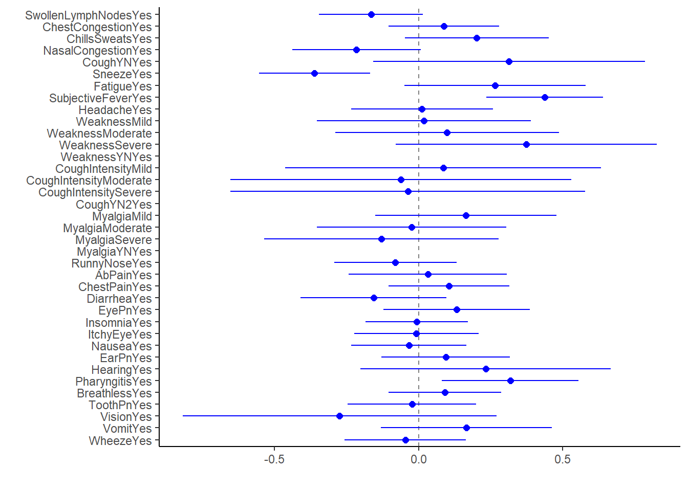

#there's a lot of information here, but hard to identify the ones that are significant due to volume

#box and whisker plot for lm_fit2 significant predictors
#first filter significant results
lm_fit2_sig <- broom.mixed::tidy(lm_fit2) %>%
                  dplyr::filter(p.value < 0.05)

#box and whisker plot for lm_fit2 significant predictors
lm_fit2_bp2 <- lm_fit2_sig %>%
                  dotwhisker::dwplot(dot_args = list(size = 2, color = "blue"),
                                     whisker_args = list(color = "blue"),
                                     vline = geom_vline(xintercept = 0, colour = "grey50", linetype = 2))
lm_fit2_bp2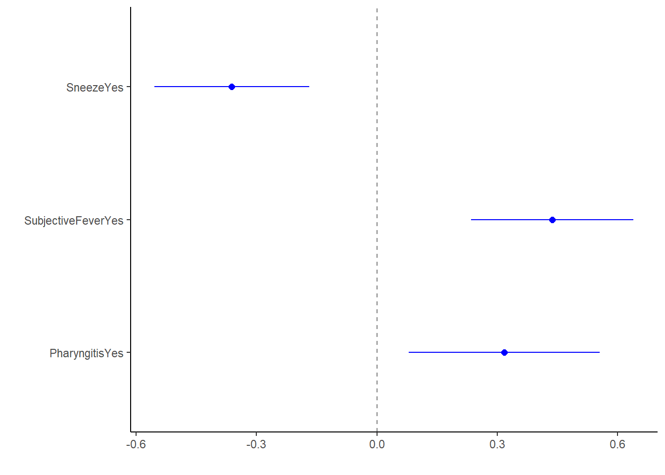

Last, we can use the glance function to examine goodness of fit measures

lm_fit2_gf <- modelsummary::glance(lm_fit2)
lm_fit2_gf

## # A tibble: 1 x 12
##   r.squared adj.r.squared sigma statistic      p.value    df logLik   AIC   BIC
##       <dbl>         <dbl> <dbl>     <dbl>        <dbl> <dbl>  <dbl> <dbl> <dbl>
## 1     0.129        0.0860  1.14      3.02 0.0000000420    34 -1116. 2304. 2469.
## # ... with 3 more variables: deviance <dbl>, df.residual <int>, nobs <int>

In comparison to lm_fit1, this model has an increased R^2, slightly lower AIC, BIC, but we need the formal comparison to better understand the significance.

Compare the Linear Regression Models

First, we want to combine results of the two models into one table.

#create a list of the two models
lm_models <- list(lm_fit1, lm_fit2)

#using the model summary package
#list estimate, 95% confidence intervals, and highlight ones with significant p-values
#hide intercept estimate
modelsummary::modelsummary(lm_models, 
                           stars = TRUE, 
                           fmt = '%.3f',
                           estimate  = "{estimate} [{conf.low}, {conf.high}] {stars}",
                           statistic = NULL,
                           coef_omit = "Intercept")

## Warning: In version 0.8.0 of the `modelsummary` package, the default significance markers produced by the `stars=TRUE` argument were changed to be consistent with R's defaults.
## This warning is displayed once per session.

	Model 1	Model 2
RunnyNoseYes	-0.293 [-0.483, -0.102] **	-0.080 [-0.294, 0.133]
SwollenLymphNodesYes		-0.165 [-0.346, 0.015] +
ChestCongestionYes		0.087 [-0.104, 0.279]
ChillsSweatsYes		0.201 [-0.049, 0.451]
NasalCongestionYes		-0.216 [-0.439, 0.008] +
CoughYNYes		0.314 [-0.159, 0.787]
SneezeYes		-0.362 [-0.555, -0.169] ***
FatigueYes		0.265 [-0.050, 0.580] +
SubjectiveFeverYes		0.437 [0.234, 0.640] ***
HeadacheYes		0.011 [-0.235, 0.258]
WeaknessMild		0.018 [-0.353, 0.390]
WeaknessModerate		0.099 [-0.290, 0.487]
WeaknessSevere		0.373 [-0.080, 0.827]
WeaknessYNYes
CoughIntensityMild		0.085 [-0.465, 0.634]
CoughIntensityModerate		-0.061 [-0.654, 0.532]
CoughIntensitySevere		-0.037 [-0.654, 0.579]
CoughYN2Yes
MyalgiaMild		0.164 [-0.151, 0.479]
MyalgiaModerate		-0.024 [-0.354, 0.305]
MyalgiaSevere		-0.129 [-0.537, 0.279]
MyalgiaYNYes
AbPainYes		0.032 [-0.244, 0.307]
ChestPainYes		0.105 [-0.105, 0.315]
DiarrheaYes		-0.157 [-0.411, 0.098]
EyePnYes		0.132 [-0.123, 0.386]
InsomniaYes		-0.007 [-0.185, 0.171]
ItchyEyeYes		-0.008 [-0.224, 0.208]
NauseaYes		-0.034 [-0.234, 0.166]
EarPnYes		0.094 [-0.130, 0.317]
HearingYes		0.232 [-0.204, 0.668]
PharyngitisYes		0.318 [0.079, 0.556] **
BreathlessYes		0.091 [-0.105, 0.287]
ToothPnYes		-0.023 [-0.246, 0.200]
VisionYes		-0.275 [-0.820, 0.271]
VomitYes		0.165 [-0.132, 0.463]
WheezeYes		-0.047 [-0.257, 0.163]
Num.Obs.	730	730
R2	0.012	0.129
R2 Adj.	0.011	0.086
AIC	2329.3	2303.8
BIC	2343.1	2469.2
Log.Lik.	-1161.673	-1115.920

In this comparison, we can see the significance of the runny nose estimate decreases, the runny nose Beta estimate gets closer to zero. Moreover, in comparison to lm_fit1, lm_fit2 has increased R^2, slightly lower AIC, BIC, log likelihood.

Next, we can conduct an ANOVA to formally compare the two linear regression models

lm_anova <- anova(lm_fit1$fit, lm_fit2$fit, test = "Chisq")
lm_anova

## Analysis of Variance Table
## 
## Model 1: BodyTemp ~ RunnyNose
## Model 2: BodyTemp ~ SwollenLymphNodes + ChestCongestion + ChillsSweats + 
##     NasalCongestion + CoughYN + Sneeze + Fatigue + SubjectiveFever + 
##     Headache + Weakness + WeaknessYN + CoughIntensity + CoughYN2 + 
##     Myalgia + MyalgiaYN + RunnyNose + AbPain + ChestPain + Diarrhea + 
##     EyePn + Insomnia + ItchyEye + Nausea + EarPn + Hearing + 
##     Pharyngitis + Breathless + ToothPn + Vision + Vomit + Wheeze
##   Res.Df     RSS Df Sum of Sq     Pr(>Chi)    
## 1    728 1030.53                              
## 2    695  909.12 33    121.41 0.0000001357 ***
## ---
## Signif. codes:  0 '***' 0.001 '**' 0.01 '*' 0.05 '.' 0.1 ' ' 1

Based on the p-value from the ANOVA, we can conclude the more complex model better describes the data than the SLR. This is also supported by the comparison of AIC and BIC above.

Logistic Model for Nausea with Runny Nose

The next model to create is a simple one using the categorical outcome of interest (Nausea) and main predictor of interest (RunnyNose). Using the parsnip package, specify the functional form of the model (logistic regression) and method for fitting the model, aka engine (“glm”)

#save the model object as log_mod
log_mod <-
  parsnip::logistic_reg() %>%
  parsnip::set_engine("glm")

We can now estimate the model using the fit function.

log_fit1 <- log_mod %>%
  fit(Nausea ~ RunnyNose, data = mydata)

Next, we can summarize logistic model with the tidy function. However, we want to exponentiate estimates to make them interpretable odds ratios.

log_fit1_summary <- broom.mixed::tidy(log_fit1, exponentiate = TRUE)
log_fit1_summary

## # A tibble: 2 x 5
##   term         estimate std.error statistic    p.value
##   <chr>           <dbl>     <dbl>     <dbl>      <dbl>
## 1 (Intercept)     0.518     0.145    -4.53  0.00000589
## 2 RunnyNoseYes    1.05      0.172     0.292 0.770

This does not yield a significant estimate (p > 0.05).

Now, we can create a box and whisker plot for log_fit1 output.

log_fit1_bp <- broom.mixed::tidy(log_fit1) %>%
                dotwhisker::dwplot(dot_args = list(size = 2, color = "blue"),
                                   whisker_args = list(color = "blue"),
                                   vline = geom_vline(xintercept = 0, colour = "grey50", linetype = 2))
log_fit1_bp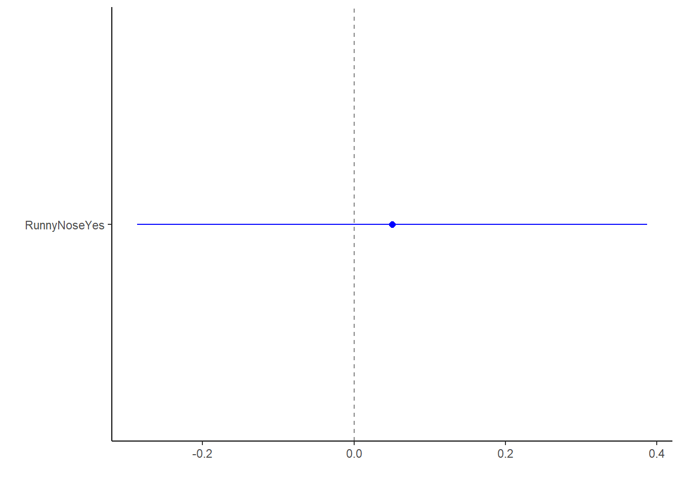

This doesn’t really mean much since we only have one category beyond not significant results.

Lastly, we can use the glance function to examine goodness of fit measures.

log_fit1_gf <-modelsummary::glance(log_fit1)
log_fit1_gf

## # A tibble: 1 x 8
##   null.deviance df.null logLik   AIC   BIC deviance df.residual  nobs
##           <dbl>   <int>  <dbl> <dbl> <dbl>    <dbl>       <int> <int>
## 1          945.     729  -472.  949.  958.     945.         728   730

We can see this fit has a lower AIC, BIC, loglikelihood than linear model. This is obviously not a direct comparison but still an interesting result.

Logistic Model for Nausea with All Predictors

The second logistic model to create includes all variables in the dataset as predictors with the main outcome of interest as Nausea. We can use the same log_mod function, so no need to respecify. We first want to create model including all predictors (defined using the . instead of specifying all variable names).

#doesn't include interaction terms
log_fit2 <- log_mod %>%
  fit(Nausea ~ ., data = mydata)

Next, we can summarize logistic model with the tidy function. However, we want to exponentiate estimates to make them interpretable odds ratios.

#adding the print function to see all rows
log_fit2_summary <- print(broom.mixed::tidy(log_fit2, exponentiate = TRUE), n = 38)

## # A tibble: 38 x 5
##    term                   estimate std.error statistic   p.value
##    <chr>                     <dbl>     <dbl>     <dbl>     <dbl>
##  1 (Intercept)               1.25     7.83      0.0285  9.77e- 1
##  2 SwollenLymphNodesYes      0.778    0.196    -1.28    2.00e- 1
##  3 ChestCongestionYes        1.32     0.213     1.30    1.95e- 1
##  4 ChillsSweatsYes           1.32     0.288     0.952   3.41e- 1
##  5 NasalCongestionYes        1.53     0.255     1.67    9.44e- 2
##  6 CoughYNYes                0.869    0.519    -0.271   7.87e- 1
##  7 SneezeYes                 1.19     0.210     0.840   4.01e- 1
##  8 FatigueYes                1.26     0.372     0.616   5.38e- 1
##  9 SubjectiveFeverYes        1.32     0.225     1.23    2.18e- 1
## 10 HeadacheYes               1.39     0.285     1.16    2.45e- 1
## 11 WeaknessMild              0.885    0.447    -0.272   7.86e- 1
## 12 WeaknessModerate          1.36     0.454     0.684   4.94e- 1
## 13 WeaknessSevere            2.28     0.510     1.61    1.07e- 1
## 14 WeaknessYNYes            NA       NA        NA      NA       
## 15 CoughIntensityMild        0.802    0.584    -0.378   7.06e- 1
## 16 CoughIntensityModerate    0.696    0.631    -0.574   5.66e- 1
## 17 CoughIntensitySevere      0.387    0.658    -1.44    1.49e- 1
## 18 CoughYN2Yes              NA       NA        NA      NA       
## 19 MyalgiaMild               0.996    0.368    -0.0113  9.91e- 1
## 20 MyalgiaModerate           1.23     0.373     0.549   5.83e- 1
## 21 MyalgiaSevere             1.13     0.445     0.271   7.86e- 1
## 22 MyalgiaYNYes             NA       NA        NA      NA       
## 23 RunnyNoseYes              1.05     0.233     0.195   8.46e- 1
## 24 AbPainYes                 2.56     0.281     3.34    8.46e- 4
## 25 ChestPainYes              1.07     0.228     0.311   7.56e- 1
## 26 DiarrheaYes               2.90     0.259     4.11    3.91e- 5
## 27 EyePnYes                  0.710    0.278    -1.23    2.18e- 1
## 28 InsomniaYes               1.09     0.193     0.436   6.63e- 1
## 29 ItchyEyeYes               0.939    0.233    -0.273   7.85e- 1
## 30 EarPnYes                  0.834    0.239    -0.760   4.47e- 1
## 31 HearingYes                1.38     0.452     0.714   4.75e- 1
## 32 PharyngitisYes            1.32     0.266     1.03    3.01e- 1
## 33 BreathlessYes             1.69     0.209     2.53    1.15e- 2
## 34 ToothPnYes                1.62     0.229     2.09    3.62e- 2
## 35 VisionYes                 1.13     0.541     0.232   8.17e- 1
## 36 VomitYes                 11.7      0.349     7.05    1.76e-12
## 37 WheezeYes                 0.738    0.234    -1.30    1.93e- 1
## 38 BodyTemp                  0.969    0.0798   -0.391   6.96e- 1

log_fit2_summary

## # A tibble: 38 x 5
##    term                 estimate std.error statistic p.value
##    <chr>                   <dbl>     <dbl>     <dbl>   <dbl>
##  1 (Intercept)             1.25      7.83     0.0285  0.977 
##  2 SwollenLymphNodesYes    0.778     0.196   -1.28    0.200 
##  3 ChestCongestionYes      1.32      0.213    1.30    0.195 
##  4 ChillsSweatsYes         1.32      0.288    0.952   0.341 
##  5 NasalCongestionYes      1.53      0.255    1.67    0.0944
##  6 CoughYNYes              0.869     0.519   -0.271   0.787 
##  7 SneezeYes               1.19      0.210    0.840   0.401 
##  8 FatigueYes              1.26      0.372    0.616   0.538 
##  9 SubjectiveFeverYes      1.32      0.225    1.23    0.218 
## 10 HeadacheYes             1.39      0.285    1.16    0.245 
## # ... with 28 more rows

#the NA lines are where all patients are reporting the symptom (so no comparison possibility)

#export results into a table using the gtsummary package
log_fit2_gtsummary <- gtsummary::tbl_regression(log_fit2, exponentiate = TRUE)

## Extracting {parsnip} model fit with `tbl_regression(x = x$fit, ...)`

log_fit2_gtsummary

Characteristic	OR¹	95% CI¹	p-value
SwollenLymphNodes
No	—	—
Yes	0.78	0.53, 1.14	0.2
ChestCongestion
No	—	—
Yes	1.32	0.87, 2.00	0.2
ChillsSweats
No	—	—
Yes	1.32	0.75, 2.34	0.3
NasalCongestion
No	—	—
Yes	1.53	0.94, 2.54	0.094
CoughYN
No	—	—
Yes	0.87	0.32, 2.49	0.8
Sneeze
No	—	—
Yes	1.19	0.79, 1.81	0.4
Fatigue
No	—	—
Yes	1.26	0.62, 2.69	0.5
SubjectiveFever
No	—	—
Yes	1.32	0.85, 2.06	0.2
Headache
No	—	—
Yes	1.39	0.81, 2.47	0.2
Weakness
None	—	—
Mild	0.89	0.38, 2.22	0.8
Moderate	1.36	0.58, 3.47	0.5
Severe	2.28	0.86, 6.42	0.11
WeaknessYN
No	—	—
Yes
CoughIntensity
None	—	—
Mild	0.80	0.25, 2.49	0.7
Moderate	0.70	0.20, 2.37	0.6
Severe	0.39	0.10, 1.38	0.15
CoughYN2
No	—	—
Yes
Myalgia
None	—	—
Mild	1.00	0.49, 2.09	>0.9
Moderate	1.23	0.60, 2.61	0.6
Severe	1.13	0.48, 2.73	0.8
MyalgiaYN
No	—	—
Yes
RunnyNose
No	—	—
Yes	1.05	0.66, 1.66	0.8
AbPain
No	—	—
Yes	2.56	1.48, 4.47	<0.001
ChestPain
No	—	—
Yes	1.07	0.68, 1.67	0.8
Diarrhea
No	—	—
Yes	2.90	1.75, 4.83	<0.001
EyePn
No	—	—
Yes	0.71	0.41, 1.22	0.2
Insomnia
No	—	—
Yes	1.09	0.75, 1.59	0.7
ItchyEye
No	—	—
Yes	0.94	0.59, 1.48	0.8
EarPn
No	—	—
Yes	0.83	0.52, 1.33	0.4
Hearing
No	—	—
Yes	1.38	0.56, 3.33	0.5
Pharyngitis
No	—	—
Yes	1.32	0.79, 2.24	0.3
Breathless
No	—	—
Yes	1.69	1.12, 2.55	0.012
ToothPn
No	—	—
Yes	1.62	1.03, 2.54	0.036
Vision
No	—	—
Yes	1.13	0.38, 3.29	0.8
Vomit
No	—	—
Yes	11.7	6.07, 24.0	<0.001
Wheeze
No	—	—
Yes	0.74	0.46, 1.16	0.2
BodyTemp	0.97	0.83, 1.13	0.7
¹ OR = Odds Ratio, CI = Confidence Interval

In this model, the significant predictors at alpha = 0.05 are AbPain, Diarrhea, Breathless, ToothPn, and Vomit. Vomit and Diarrhea makes sense as they often co-present with nausea, and abdominal pain as well as breathlessness make clinical sense. Tooth pain is a surprising result.

Now we can create a box and whisker plot for log_fit2 output.

log_fit2_bp1 <- broom.mixed::tidy(log_fit2) %>%
                  dotwhisker::dwplot(dot_args = list(size = 2, color = "blue"),
                                     whisker_args = list(color = "blue"),
                                     vline = geom_vline(xintercept = 0, colour = "grey50", linetype = 2))
log_fit2_bp1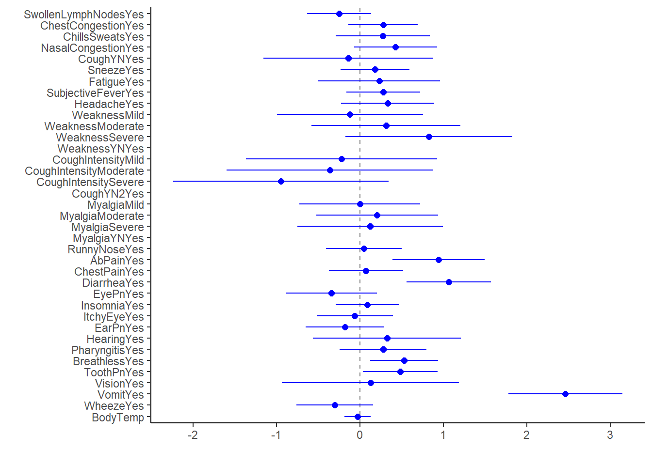

#there's a lot of information here, but hard to identify the ones that are significant due to volume

#box and whisker plot for log_fit2 significant predictors
#first filter significant results
log_fit2_sig <- broom.mixed::tidy(log_fit2) %>%
  dplyr::filter(p.value < 0.05)

#box and whisker plot for log_fit2 significant predictors
log_fit2_bp2 <- log_fit2_sig %>%
                  dotwhisker::dwplot(dot_args = list(size = 2, color = "blue"),
                                     whisker_args = list(color = "blue"),
                                     vline = geom_vline(xintercept = 0, colour = "grey50", linetype = 2))
log_fit2_bp2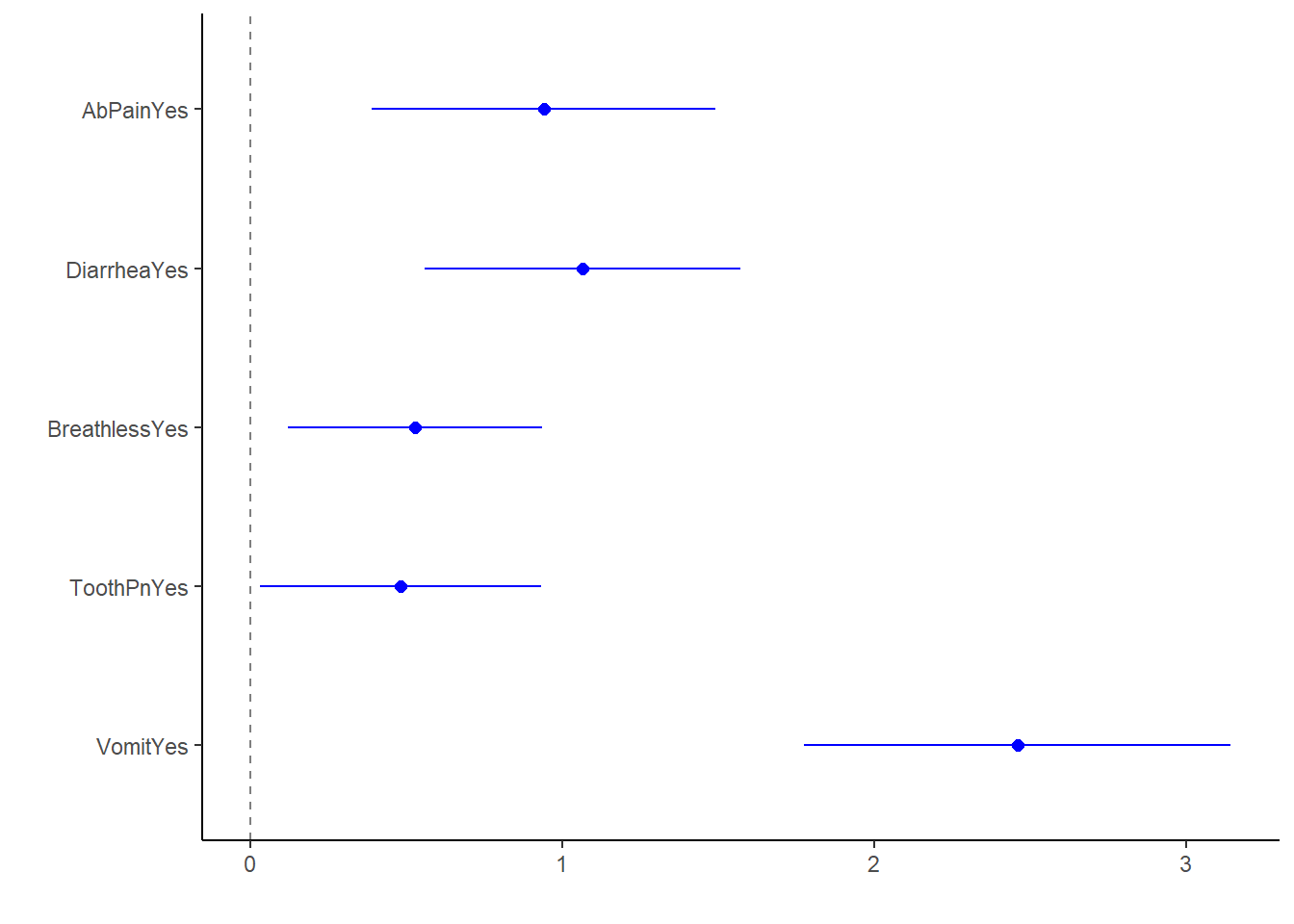

All significant predictors in this model increase odds of having nausea. It makes sense vomit and diarrhea have the highest OR, given the frequent co-presentation of the three symptoms.

Lastly, we can use the glance function to examine goodness of fit measures.

log_fit2_gf <- modelsummary::glance(log_fit2)
log_fit2_gf

## # A tibble: 1 x 8
##   null.deviance df.null logLik   AIC   BIC deviance df.residual  nobs
##           <dbl>   <int>  <dbl> <dbl> <dbl>    <dbl>       <int> <int>
## 1          945.     729  -376.  821.  982.     751.         695   730

In comparison to log_fit1, this model has a lower log likelihood, AIC, BIC, deviance, but we need the formal comparison to better understand the significance.

Compare the Logistic Regression Models

First, we need to combine results of the two models into one table.

log_models <- list(log_fit1, log_fit2)

#list estimate, 95% confidence intervals, and highlight ones with significant p-values
#hide intercept estimate
modelsummary::modelsummary(log_models, 
                           stars = TRUE, 
                           fmt = '%.3f', 
                           exponentiate = TRUE,
                           estimate  = "{estimate} [{conf.low}, {conf.high}] {stars}",
                           statistic = NULL,
                           coef_omit = "Intercept")

	Model 1	Model 2
RunnyNoseYes	1.051 [0.753, 1.477]	1.046 [0.664, 1.656]
SwollenLymphNodesYes		0.778 [0.528, 1.140]
ChestCongestionYes		1.317 [0.869, 2.003]
ChillsSweatsYes		1.315 [0.755, 2.339]
NasalCongestionYes		1.531 [0.935, 2.541] +
CoughYNYes		0.869 [0.321, 2.487]
SneezeYes		1.193 [0.791, 1.805]
FatigueYes		1.257 [0.621, 2.693]
SubjectiveFeverYes		1.320 [0.851, 2.063]
HeadacheYes		1.393 [0.806, 2.473]
WeaknessMild		0.885 [0.380, 2.219]
WeaknessModerate		1.365 [0.577, 3.474]
WeaknessSevere		2.278 [0.859, 6.423]
WeaknessYNYes
CoughIntensityMild		0.802 [0.249, 2.494]
CoughIntensityModerate		0.696 [0.197, 2.368]
CoughIntensitySevere		0.387 [0.104, 1.384]
CoughYN2Yes
MyalgiaMild		0.996 [0.491, 2.092]
MyalgiaModerate		1.227 [0.600, 2.607]
MyalgiaSevere		1.128 [0.475, 2.733]
MyalgiaYNYes
AbPainYes		2.558 [1.478, 4.469] ***
ChestPainYes		1.073 [0.685, 1.675]
DiarrheaYes		2.898 [1.749, 4.834] ***
EyePnYes		0.710 [0.408, 1.215]
InsomniaYes		1.088 [0.745, 1.590]
ItchyEyeYes		0.939 [0.592, 1.476]
EarPnYes		0.834 [0.519, 1.327]
HearingYes		1.381 [0.558, 3.328]
PharyngitisYes		1.317 [0.788, 2.242]
BreathlessYes		1.694 [1.125, 2.551] *
ToothPnYes		1.617 [1.030, 2.536] *
VisionYes		1.134 [0.385, 3.294]
VomitYes		11.687 [6.072, 23.999] ***
WheezeYes		0.738 [0.464, 1.162]
BodyTemp		0.969 [0.827, 1.132]
Num.Obs.	730	730
AIC	948.6	821.5
BIC	957.8	982.2
Log.Lik.	-472.283	-375.735

Interestingly, runny nose is not a significant predictor in either model. In comparison to log_fit1, log_fit2 has a slightly lower AIC and log likelihood, but higher BIC.

Next, we can conduct an ANOVA to compare the two linear regression models

log_anova <- anova(log_fit1$fit, log_fit2$fit, test = "Chisq")
log_anova

## Analysis of Deviance Table
## 
## Model 1: Nausea ~ RunnyNose
## Model 2: Nausea ~ SwollenLymphNodes + ChestCongestion + ChillsSweats + 
##     NasalCongestion + CoughYN + Sneeze + Fatigue + SubjectiveFever + 
##     Headache + Weakness + WeaknessYN + CoughIntensity + CoughYN2 + 
##     Myalgia + MyalgiaYN + RunnyNose + AbPain + ChestPain + Diarrhea + 
##     EyePn + Insomnia + ItchyEye + EarPn + Hearing + Pharyngitis + 
##     Breathless + ToothPn + Vision + Vomit + Wheeze + BodyTemp
##   Resid. Df Resid. Dev Df Deviance              Pr(>Chi)    
## 1       728     944.57                                      
## 2       695     751.47 33   193.09 < 0.00000000000000022 ***
## ---
## Signif. codes:  0 '***' 0.001 '**' 0.01 '*' 0.05 '.' 0.1 ' ' 1

Based on the p-value from the ANOVA, we can conclude the more complex model better describes the data than the simple logistic regression, which is also supported by the comparison of measures above. However, the higher BIC suggests the significance noted may be a result from the number of parameters included in the model. In a real-world analysis, we would need to examine the potential of overfitting occurring in the full logistic regression model.