Influenza Project - Machine Learning Models

Introduction

This exercise fits three machine learning models to the influenza data: decision tree, LASSO, and random forest. It compares the three chosen models, and then finally fits the “best” model to the test data.

The raw data for this exercise comes from the following citation: McKay, Brian et al. (2020), Virulence-mediated infectiousness and activity trade-offs and their impact on transmission potential of patients infected with influenza, Dryad, Dataset, https://doi.org/10.5061/dryad.51c59zw4v.

The processed data was produced on the Data Processing tab.

Within this analysis, the following definitions exist:

Main predictor of interest = Runny Nose
Continuous outcome of interest = Body Temperature

Each machine learning model will be follow this process:

Model Specification
Workflow Definition
Tuning Grid Specification
Tuning Using Cross-Validation and the tune_grid() function
Identify Best Model
Model Evaluation

Required Packages

The following R packages are required for this exercise:

here: for data loading/saving
tidyverse: for data management
tidymodels: for data modeling
skimr: for variable summaries
broom.mixed: for converting bayesian models to tidy tibbles
rpart.plot: for visualizing a decision tree
vip: for variable importance plots
glmnet: for lasso models
doParallel: for parallel backend for tuning processes
ranger: for random forest models

Load Data

Load the processed data from the processed_data folder in the project file.

#path to data
#note the use of the here() package and not absolute paths
data_location <- here::here("data","flu","ML_data.rds")

#load data. 
ML_processed <- readRDS(data_location)

#summary of data using skimr package
skimr::skim(ML_processed)

Data summary
Name	ML_processed
Number of rows	730
Number of columns	26
_______________________
Column type frequency:
factor	25
numeric	1
________________________
Group variables	None

Variable type: factor

skim_variable	complete_rate	ordered	n_unique	top_counts
SwollenLymphNodes	1	FALSE	2	No: 418, Yes: 312
ChestCongestion	1	FALSE	2	Yes: 407, No: 323
ChillsSweats	1	FALSE	2	Yes: 600, No: 130
NasalCongestion	1	FALSE	2	Yes: 563, No: 167
Sneeze	1	FALSE	2	Yes: 391, No: 339
Fatigue	1	FALSE	2	Yes: 666, No: 64
SubjectiveFever	1	FALSE	2	Yes: 500, No: 230
Headache	1	FALSE	2	Yes: 615, No: 115
Weakness	1	TRUE	4	Mod: 338, Mil: 223, Sev: 120, Non: 49
CoughIntensity	1	TRUE	4	Mod: 357, Sev: 172, Mil: 154, Non: 47
Myalgia	1	TRUE	4	Mod: 325, Mil: 213, Sev: 113, Non: 79
RunnyNose	1	FALSE	2	Yes: 519, No: 211
AbPain	1	FALSE	2	No: 639, Yes: 91
ChestPain	1	FALSE	2	No: 497, Yes: 233
Diarrhea	1	FALSE	2	No: 631, Yes: 99
EyePn	1	FALSE	2	No: 617, Yes: 113
Insomnia	1	FALSE	2	Yes: 415, No: 315
ItchyEye	1	FALSE	2	No: 551, Yes: 179
Nausea	1	FALSE	2	No: 475, Yes: 255
EarPn	1	FALSE	2	No: 568, Yes: 162
Pharyngitis	1	FALSE	2	Yes: 611, No: 119
Breathless	1	FALSE	2	No: 436, Yes: 294
ToothPn	1	FALSE	2	No: 565, Yes: 165
Vomit	1	FALSE	2	No: 652, Yes: 78
Wheeze	1	FALSE	2	No: 510, Yes: 220

Variable type: numeric

skim_variable	n_missing	complete_rate	mean	sd	p0	p25	p50	p75	p100	hist
BodyTemp	0	1	98.94	1.2	97.2	98.2	98.5	99.3	103.1	▇▇▂▁▁

Data Setup

Following the parameters determined in the assignment guidelines:

Set the random seed to 123
Split the dataset into 70% training, 30% testing with BodyTemp as stratification
5-fold cross validation, 5 times repeated, stratified on BodyTemp for the CV folds
Create a recipe for data and fitting that codes categorical variables as dummy variables

#set random seed to 123
set.seed(123)

#split dataset into 70% training, 30% testing
#use BodyTemp as stratification
data_split <- rsample::initial_split(ML_processed, prop = 7/10,
                                     strata = BodyTemp)

#create dataframes for the two sets:
train_data <- rsample::training(data_split)
test_data <- rsample::testing(data_split)

#training set proportions by BodyTemp
train_data %>%
  dplyr::count(BodyTemp) %>%
  dplyr::mutate(prop = n / sum(n))

##    BodyTemp  n        prop
## 1      97.3  1 0.001968504
## 2      97.4  5 0.009842520
## 3      97.5  8 0.015748031
## 4      97.6  5 0.009842520
## 5      97.7 12 0.023622047
## 6      97.8 19 0.037401575
## 7      97.9 23 0.045275591
## 8      98.0 18 0.035433071
## 9      98.1 29 0.057086614
## 10     98.2 32 0.062992126
## 11     98.3 42 0.082677165
## 12     98.4 29 0.057086614
## 13     98.5 37 0.072834646
## 14     98.6 14 0.027559055
## 15     98.7 28 0.055118110
## 16     98.8 15 0.029527559
## 17     98.9 13 0.025590551
## 18     99.0 21 0.041338583
## 19     99.1 11 0.021653543
## 20     99.2 15 0.029527559
## 21     99.3 13 0.025590551
## 22     99.4 10 0.019685039
## 23     99.5  8 0.015748031
## 24     99.6  3 0.005905512
## 25     99.7  6 0.011811024
## 26     99.8  5 0.009842520
## 27     99.9  9 0.017716535
## 28    100.0  5 0.009842520
## 29    100.1  4 0.007874016
## 30    100.2  5 0.009842520
## 31    100.3  4 0.007874016
## 32    100.4  5 0.009842520
## 33    100.5  3 0.005905512
## 34    100.6  2 0.003937008
## 35    100.8  1 0.001968504
## 36    100.9  7 0.013779528
## 37    101.0  1 0.001968504
## 38    101.1  3 0.005905512
## 39    101.2  3 0.005905512
## 40    101.3  1 0.001968504
## 41    101.5  1 0.001968504
## 42    101.6  2 0.003937008
## 43    101.7  3 0.005905512
## 44    101.8  1 0.001968504
## 45    101.9  3 0.005905512
## 46    102.0  2 0.003937008
## 47    102.1  1 0.001968504
## 48    102.2  2 0.003937008
## 49    102.4  1 0.001968504
## 50    102.5  1 0.001968504
## 51    102.6  2 0.003937008
## 52    102.7  2 0.003937008
## 53    102.8  4 0.007874016
## 54    103.0  6 0.011811024
## 55    103.1  2 0.003937008

#testing set proportions by BodyTemp
test_data %>%
  dplyr::count(BodyTemp) %>%
  dplyr::mutate(prop = n / sum(n))

##    BodyTemp  n        prop
## 1      97.2  2 0.009009009
## 2      97.4  2 0.009009009
## 3      97.5  1 0.004504505
## 4      97.6  2 0.009009009
## 5      97.7  2 0.009009009
## 6      97.8  4 0.018018018
## 7      97.9  6 0.027027027
## 8      98.0 12 0.054054054
## 9      98.1 17 0.076576577
## 10     98.2 18 0.081081081
## 11     98.3 20 0.090090090
## 12     98.4 11 0.049549550
## 13     98.5 16 0.072072072
## 14     98.6 13 0.058558559
## 15     98.7  7 0.031531532
## 16     98.8  9 0.040540541
## 17     98.9 10 0.045045045
## 18     99.0  4 0.018018018
## 19     99.1  4 0.018018018
## 20     99.2  5 0.022522523
## 21     99.3  5 0.022522523
## 22     99.4  1 0.004504505
## 23     99.5  6 0.027027027
## 24     99.6  3 0.013513514
## 25     99.7  5 0.022522523
## 26     99.8  1 0.004504505
## 27     99.9  1 0.004504505
## 28    100.0  2 0.009009009
## 29    100.1  3 0.013513514
## 30    100.2  3 0.013513514
## 31    100.3  1 0.004504505
## 32    100.4  2 0.009009009
## 33    100.5  2 0.009009009
## 34    100.6  2 0.009009009
## 35    100.8  1 0.004504505
## 36    100.9  2 0.009009009
## 37    101.0  1 0.004504505
## 38    101.2  1 0.004504505
## 39    101.5  1 0.004504505
## 40    101.8  3 0.013513514
## 41    101.9  3 0.013513514
## 42    102.1  1 0.004504505
## 43    102.2  1 0.004504505
## 44    102.4  1 0.004504505
## 45    102.5  1 0.004504505
## 46    102.6  1 0.004504505
## 47    102.8  1 0.004504505
## 48    102.9  1 0.004504505
## 49    103.0  1 0.004504505

#5-fold cross validation, 5 times repeated, stratified on `BodyTemp` for the CV folds
folds <- rsample::vfold_cv(train_data,
                           v = 5,
                           repeats = 5,
                           strata = BodyTemp)
  
#create recipe that codes categorical variables as dummy variables
flu_rec <- recipes::recipe(BodyTemp ~ ., data = train_data) %>%
           recipes::step_dummy(all_nominal_predictors())

Null model performance

Determine the performance of a null model (i.e. one with no predictors). For a continuous outcome and RMSE as the metric, a null model is one that predicts the mean of the outcome. Compute the RMSE for both training and test data for such a model.

#create null model
null_mod <- parsnip::null_model() %>%
            parsnip::set_engine("parsnip") %>%
            parsnip::set_mode("regression")

#add recipe and model into workflow
null_wflow <- workflows::workflow() %>%
              workflows::add_recipe(flu_rec) %>%
              workflows::add_model(null_mod)

#"fit" model to training data
null_train <- null_wflow %>%
                parsnip::fit(data = train_data)

#summary of null model with training data to get mean (which in this case is the RMSE)
null_train_sum <- broom.mixed::tidy(null_train)
null_train_sum

## # A tibble: 1 x 1
##   value
##   <dbl>
## 1  98.9

#"fit" model to test data
null_test <- null_wflow %>%
                parsnip::fit(data = test_data)

#summary of null model with test data to get mean (which in this case is the RMSE)
null_test_sum <- broom.mixed::tidy(null_test)
null_test_sum

## # A tibble: 1 x 1
##   value
##   <dbl>
## 1  98.9

#RMSE for training data
null_RMSE_train <- tibble::tibble(
                      rmse = rmse_vec(truth = train_data$BodyTemp,
                                          estimate = rep(mean(train_data$BodyTemp), nrow(train_data))),
                      SE = 0,
                      model = "Null - Train")

#RMSE for testing data
null_RMSE_test <- tibble::tibble(
                      rmse = rmse_vec(truth = test_data$BodyTemp,
                                          estimate = rep(mean(test_data$BodyTemp), nrow(test_data))),
                      SE = 0,
                      model = "Null - Test")

Tree Model

Most of the code for this section comes from the TidyModels Tutorial for Tuning.

1. Model Specification

#run parallels to determine number of cores
cores <- parallel::detectCores() - 1
cores

## [1] 19

cl <- makeCluster(cores)

registerDoParallel(cl)

#define the tree model
tree_mod <-
  parsnip::decision_tree(cost_complexity = tune(),
                         tree_depth = tune(),
                         min_n = tune()) %>%
  parsnip::set_engine("rpart") %>%
  parsnip::set_mode("regression")

#use the recipe specified earlier (line 133)

2. Workflow Definition

#define workflow for tree
tree_wflow <- workflows::workflow() %>%
               workflows::add_model(tree_mod) %>%
               workflows::add_recipe(flu_rec)

3. Tuning Grid Specification

#tuning grid specification
tree_grid <- dials::grid_regular(cost_complexity(),
                                 tree_depth(),
                                 min_n(),
                                 levels = 5)

#tree depth
tree_grid %>%
  dplyr::count(tree_depth)

## # A tibble: 5 x 2
##   tree_depth     n
##        <int> <int>
## 1          1    25
## 2          4    25
## 3          8    25
## 4         11    25
## 5         15    25

4. Tuning Using Cross-Validation and the `tune_grid()` function

#tune the model with previously specified cross-validation and RMSE as target metric
tree_res <- tree_wflow %>%
                tune::tune_grid(resamples = folds,
                                grid = tree_grid,
                                control = control_grid(verbose = TRUE),
                                metrics = yardstick::metric_set(rmse))

#collect metrics
tree_res %>% workflowsets::collect_metrics()

## # A tibble: 125 x 9
##    cost_complexity tree_depth min_n .metric .estimator  mean     n std_err
##              <dbl>      <int> <int> <chr>   <chr>      <dbl> <int>   <dbl>
##  1    0.0000000001          1     2 rmse    standard    1.19    25  0.0181
##  2    0.0000000178          1     2 rmse    standard    1.19    25  0.0181
##  3    0.00000316            1     2 rmse    standard    1.19    25  0.0181
##  4    0.000562              1     2 rmse    standard    1.19    25  0.0181
##  5    0.1                   1     2 rmse    standard    1.21    25  0.0177
##  6    0.0000000001          4     2 rmse    standard    1.24    25  0.0204
##  7    0.0000000178          4     2 rmse    standard    1.24    25  0.0204
##  8    0.00000316            4     2 rmse    standard    1.24    25  0.0204
##  9    0.000562              4     2 rmse    standard    1.23    25  0.0205
## 10    0.1                   4     2 rmse    standard    1.21    25  0.0177
## # ... with 115 more rows, and 1 more variable: .config <chr>

#default visualization
tree_res %>% autoplot()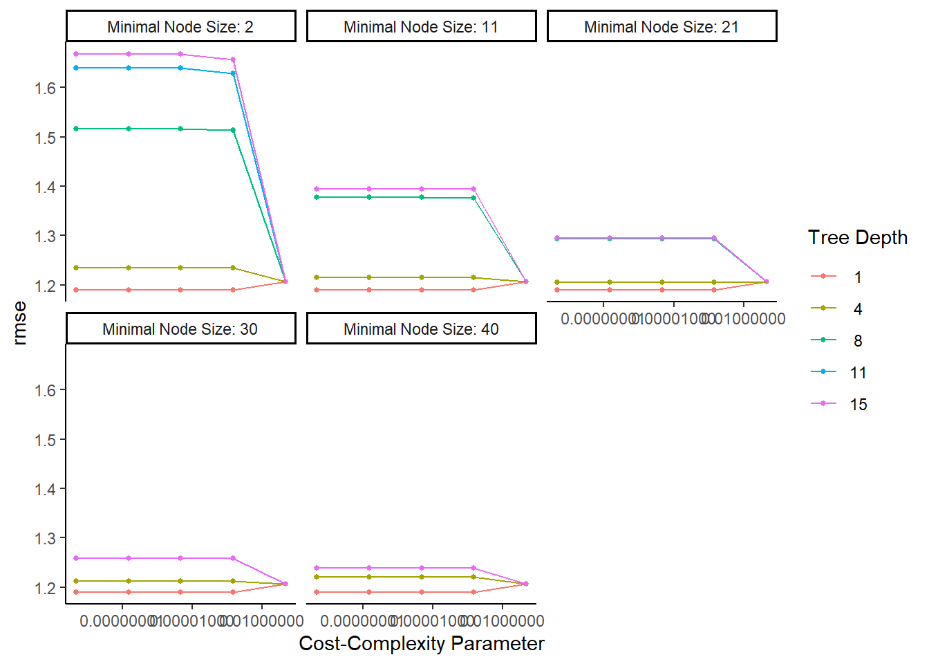

#more detailed plot
tree_res %>%
  workflowsets::collect_metrics() %>%
  dplyr::mutate(tree_depth = factor(tree_depth)) %>%
  ggplot2::ggplot(aes(cost_complexity, mean, color = tree_depth)) +
           geom_line(size = 1.5, alpha = 0.6) +
           geom_point(size = 2) +
           facet_wrap(~ .metric, scales = "free", nrow = 2) +
           scale_x_log10(labels = scales::label_number()) +
           scale_color_viridis_d(option = "plasma", begin = 0.9, end = 0)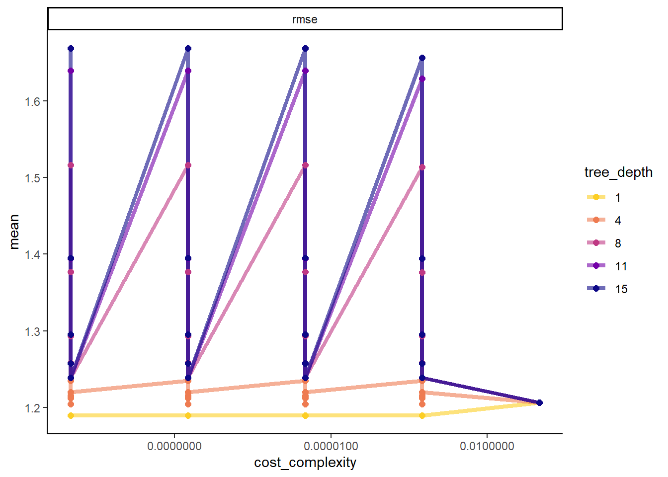

5. Identify Best Model

#select the tree model with the lowest rmse
tree_lowest_rmse <- tree_res %>%
                        tune::select_best("rmse")

#finalize the workflow by using the selected lasso model
best_tree_wflow <- tree_wflow %>%
                      tune::finalize_workflow(tree_lowest_rmse)
best_tree_wflow

## == Workflow ====================================================================
## Preprocessor: Recipe
## Model: decision_tree()
## 
## -- Preprocessor ----------------------------------------------------------------
## 1 Recipe Step
## 
## * step_dummy()
## 
## -- Model -----------------------------------------------------------------------
## Decision Tree Model Specification (regression)
## 
## Main Arguments:
##   cost_complexity = 0.0000000001
##   tree_depth = 1
##   min_n = 2
## 
## Computational engine: rpart

#one last fit on the training data
best_tree_fit <- best_tree_wflow %>%
                    parsnip::fit(data = train_data)

6. Model evaluation

#plot the tree
rpart.plot::rpart.plot(x = workflowsets::extract_fit_parsnip(best_tree_fit)$fit,
                       roundint = F,
                       type = 5,
                       digits = 5,
                       main = "Selected Tree Model")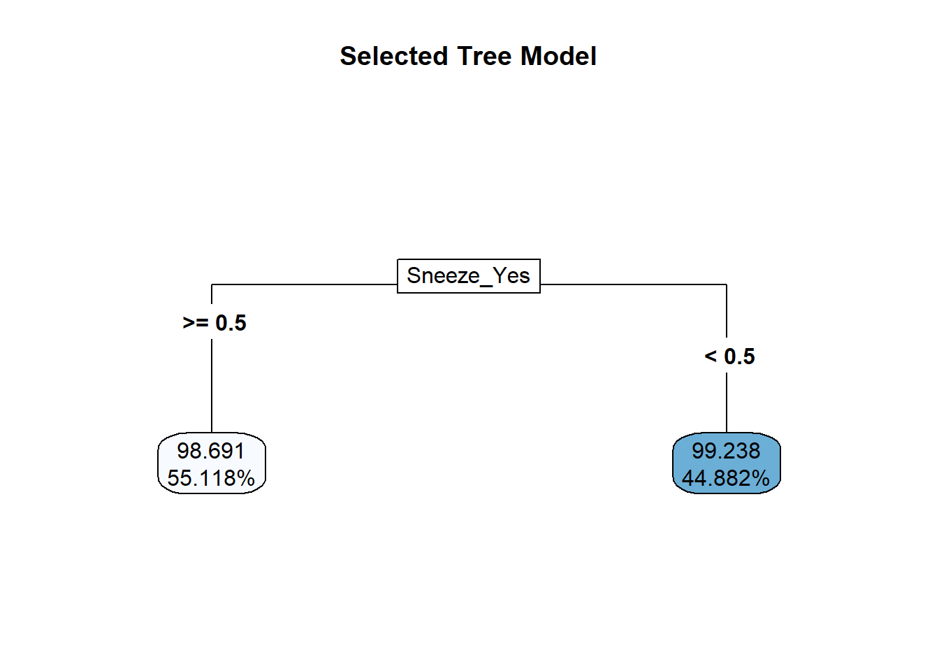

#find predictions and intervals
tree_resid <- best_tree_fit %>%
                  broom.mixed::augment(new_data = train_data) %>%
                  dplyr::select(.pred, BodyTemp) %>%
                  dplyr::mutate(.resid = .pred - BodyTemp)

#plot model predictions from tuned model versus actual outcomes
#geom_abline draws a 45 degree line, along which the results should fall
ggplot2::ggplot(tree_resid, aes(x = .pred, y = BodyTemp)) +
  geom_abline(slope = 1, intercept = 0, color = "red", lty = 2) + 
  geom_point() +
  xlim(97, 104) +
  ylim (97, 104) +
  labs(title = "Decision Tree Fit: Predicted vs. Actual Body Temperature",
        x = "Predicted Body Temperature (F)",
        y = "Actual Body Temperature (F)")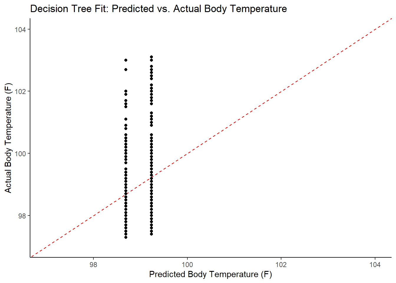

#plot model with residuals
#the geom_hline plots a straight horizontal line along which the results should fall
ggplot2::ggplot(tree_resid, aes(x = as.numeric(row.names(tree_resid)), y = .resid))+
  geom_hline(yintercept = 0, color = "red", lty = 2) +
  geom_point() +
  labs(title = "Decision Tree Fit: Residuals",
        x = "Observation Number",
        y = "Residual")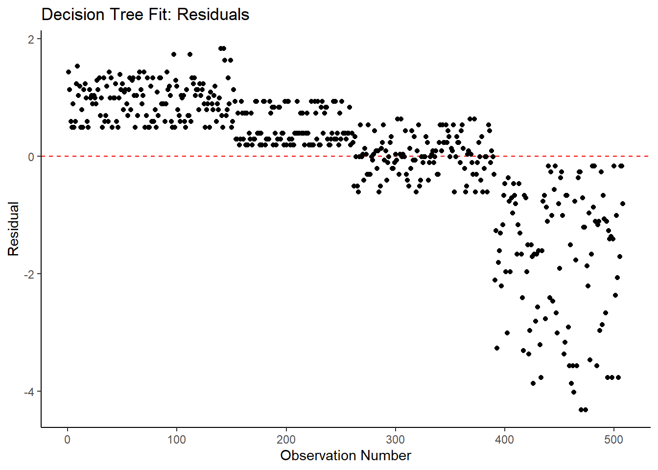

#plot model fit vs residuals
#the geom_hline plots a straight horizontal line along which the results fall
ggplot2::ggplot(tree_resid, aes(x = .pred, y = .resid))+
  geom_hline(yintercept = 0, color = "red", lty = 2) +
  geom_point() +
  xlim(97, 104) +
  labs(title = "Decision Tree Fit: Residuals vs Fitted Body Temperature",
        x = "Fitted Body Temperature (F)",
        y = "Residual")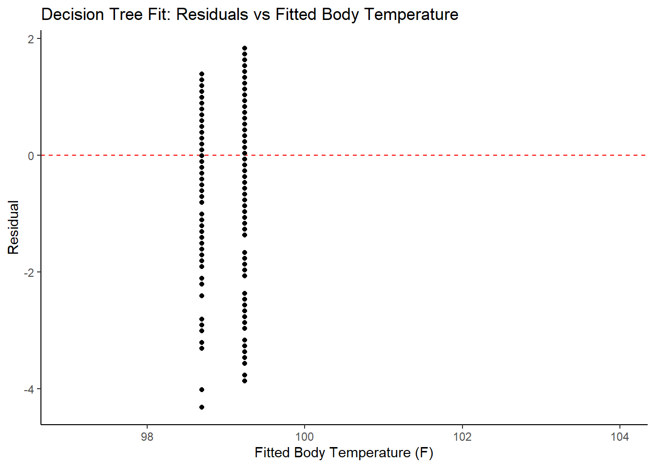

#print model performance
#print 10 best performing hyperparameter sets
tree_res %>%
  tune::show_best(n = 10) %>%
  dplyr::select(rmse = mean, std_err, cost_complexity) %>%
  dplyr::mutate(rmse = round(rmse, 3),
                std_err = round(std_err, 4),
                cost_complexity = scales::scientific(cost_complexity))

## # A tibble: 10 x 3
##     rmse std_err cost_complexity
##    <dbl>   <dbl> <chr>          
##  1  1.19  0.0181 1.00e-10       
##  2  1.19  0.0181 1.78e-08       
##  3  1.19  0.0181 3.16e-06       
##  4  1.19  0.0181 5.62e-04       
##  5  1.19  0.0181 1.00e-10       
##  6  1.19  0.0181 1.78e-08       
##  7  1.19  0.0181 3.16e-06       
##  8  1.19  0.0181 5.62e-04       
##  9  1.19  0.0181 1.00e-10       
## 10  1.19  0.0181 1.78e-08

#print the best model performance
tree_performance <- tree_res %>% tune::show_best(n = 1)
print(tree_performance)

## # A tibble: 1 x 9
##   cost_complexity tree_depth min_n .metric .estimator  mean     n std_err
##             <dbl>      <int> <int> <chr>   <chr>      <dbl> <int>   <dbl>
## 1    0.0000000001          1     2 rmse    standard    1.19    25  0.0181
## # ... with 1 more variable: .config <chr>

#compare model performance to null model
tree_RMSE <- tree_res %>%
                tune::show_best(n = 1) %>%
                dplyr::transmute(
                  rmse = round(mean, 3),
                  SE = round(std_err, 4),
                  model = "Tree") %>%
               dplyr::bind_rows(null_RMSE_train)
tree_RMSE

## # A tibble: 2 x 3
##    rmse     SE model       
##   <dbl>  <dbl> <chr>       
## 1  1.19 0.0181 Tree        
## 2  1.21 0      Null - Train

The identified best performing tree model only predicts two different values, which isn’t a great model. In comparing the RMSE to the null model, it is a marginal improvement at best. This is not a good model for this data – time to try something new!

LASSO Model

Most of the code for this section comes from the TidyModels Tutorial Case Study.

1. Model Specification

#define the lasso model
#mixture = 1 identifies the model to be a LASSO model
lasso_mod <-
  parsnip::linear_reg(mode = "regression",
                      penalty = tune(), 
                      mixture = 1) %>%
  parsnip::set_engine("glmnet")

#use the recipe specified earlier (line 133)

2. Workflow Definition

#define workflow for lasso regression
lasso_wflow <- workflows::workflow() %>%
               workflows::add_model(lasso_mod) %>%
               workflows::add_recipe(flu_rec)

3. Tuning Grid Specification

#tuning grid specification
lasso_grid <- tibble(penalty = 10^seq(-3, 0, length.out = 30))

#5 lowest penalty values
lasso_grid %>%
  dplyr::top_n(-5)

## Selecting by penalty

## # A tibble: 5 x 1
##   penalty
##     <dbl>
## 1 0.001  
## 2 0.00127
## 3 0.00161
## 4 0.00204
## 5 0.00259

#5 highest penalty values
lasso_grid %>%
  dplyr::top_n(5)

## Selecting by penalty

## # A tibble: 5 x 1
##   penalty
##     <dbl>
## 1   0.386
## 2   0.489
## 3   0.621
## 4   0.788
## 5   1

4. Tuning Using Cross-Validation and the `tune_grid()` function

#tune the model with previously specified cross-validation and RMSE as target metric
lasso_res <- lasso_wflow %>%
                tune::tune_grid(resamples = folds,
                                grid = lasso_grid,
                                control = control_grid(verbose = TRUE, 
                                                       save_pred = TRUE),
                                metrics = metric_set(rmse))

#look at 15 models with lowest RMSEs
top_lasso_models <- lasso_res %>%
                      tune::show_best("rmse", n = 15) %>%
                      dplyr::arrange(penalty)
top_lasso_models

## # A tibble: 15 x 7
##    penalty .metric .estimator  mean     n std_err .config              
##      <dbl> <chr>   <chr>      <dbl> <int>   <dbl> <chr>                
##  1 0.00530 rmse    standard    1.17    25  0.0167 Preprocessor1_Model08
##  2 0.00672 rmse    standard    1.17    25  0.0167 Preprocessor1_Model09
##  3 0.00853 rmse    standard    1.17    25  0.0167 Preprocessor1_Model10
##  4 0.0108  rmse    standard    1.17    25  0.0167 Preprocessor1_Model11
##  5 0.0137  rmse    standard    1.16    25  0.0167 Preprocessor1_Model12
##  6 0.0174  rmse    standard    1.16    25  0.0167 Preprocessor1_Model13
##  7 0.0221  rmse    standard    1.16    25  0.0168 Preprocessor1_Model14
##  8 0.0281  rmse    standard    1.16    25  0.0169 Preprocessor1_Model15
##  9 0.0356  rmse    standard    1.15    25  0.0169 Preprocessor1_Model16
## 10 0.0452  rmse    standard    1.15    25  0.0169 Preprocessor1_Model17
## 11 0.0574  rmse    standard    1.15    25  0.0169 Preprocessor1_Model18
## 12 0.0728  rmse    standard    1.15    25  0.0170 Preprocessor1_Model19
## 13 0.0924  rmse    standard    1.16    25  0.0172 Preprocessor1_Model20
## 14 0.117   rmse    standard    1.16    25  0.0175 Preprocessor1_Model21
## 15 0.149   rmse    standard    1.17    25  0.0178 Preprocessor1_Model22

#default visualization
lasso_res %>% autoplot()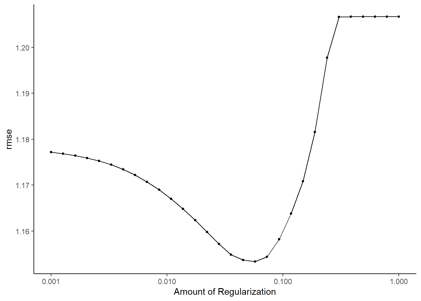

#create a graph to see when there is a significant change in the penalty
#this is the same as above, just a little more detail
lasso_res %>%
  workflowsets::collect_metrics() %>%
  ggplot2::ggplot(aes(penalty, mean, color = .metric)) +
  ggplot2::geom_errorbar(aes(ymin = mean - std_err,
                             ymax = mean + std_err),
                         alpha = 0.5) +
  ggplot2::geom_line(size = 1.5) +
  ggplot2::scale_x_log10()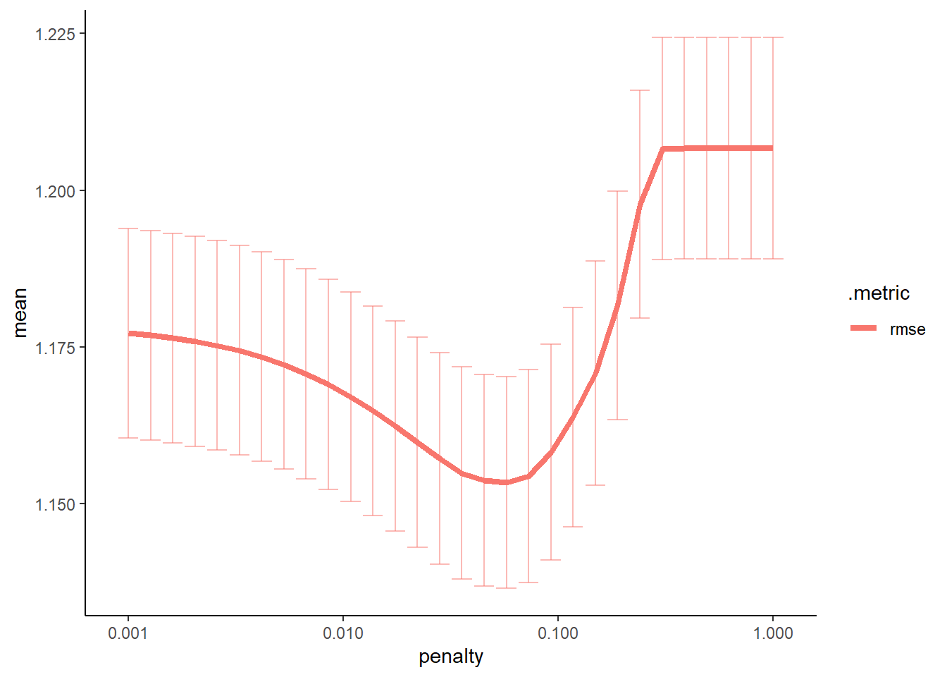

5. Identify Best Model

#select the lasso model with the lowest rmse
lasso_lowest_rmse <- lasso_res %>%
                        tune::select_best("rmse")

#finalize the workflow by using the selected lasso model
best_lasso_wflow <- lasso_wflow %>%
                      tune::finalize_workflow(lasso_lowest_rmse)
best_lasso_wflow

## == Workflow ====================================================================
## Preprocessor: Recipe
## Model: linear_reg()
## 
## -- Preprocessor ----------------------------------------------------------------
## 1 Recipe Step
## 
## * step_dummy()
## 
## -- Model -----------------------------------------------------------------------
## Linear Regression Model Specification (regression)
## 
## Main Arguments:
##   penalty = 0.0573615251044868
##   mixture = 1
## 
## Computational engine: glmnet

#one last fit on the training data
best_lasso_fit <- best_lasso_wflow %>%
                    parsnip::fit(data = train_data)

#create a table of model fit that includes the predictors in the model
#i.e. include all non-zero estimates
lasso_tibble <- best_lasso_fit %>%
                    workflowsets::extract_fit_parsnip() %>%
                    broom::tidy() %>%
                    dplyr::filter(estimate != 0) %>%
                    dplyr::mutate_if(is.numeric, round, 4)
lasso_tibble

## # A tibble: 13 x 3
##    term                estimate penalty
##    <chr>                  <dbl>   <dbl>
##  1 (Intercept)          98.7     0.0574
##  2 ChestCongestion_Yes   0.0332  0.0574
##  3 ChillsSweats_Yes      0.0894  0.0574
##  4 NasalCongestion_Yes  -0.140   0.0574
##  5 Sneeze_Yes           -0.391   0.0574
##  6 Fatigue_Yes           0.178   0.0574
##  7 SubjectiveFever_Yes   0.378   0.0574
##  8 Weakness_1            0.178   0.0574
##  9 Myalgia_2            -0.0099  0.0574
## 10 Myalgia_3             0.0679  0.0574
## 11 RunnyNose_Yes        -0.0825  0.0574
## 12 Nausea_Yes            0.0035  0.0574
## 13 Pharyngitis_Yes       0.148   0.0574

6. Model evaluation

#extract model from final fit
x_lasso <- best_lasso_fit$fit$fit$fit

#plot how number of predictors included in LASSO model changes with the tuning parameter
plot(x_lasso, "lambda")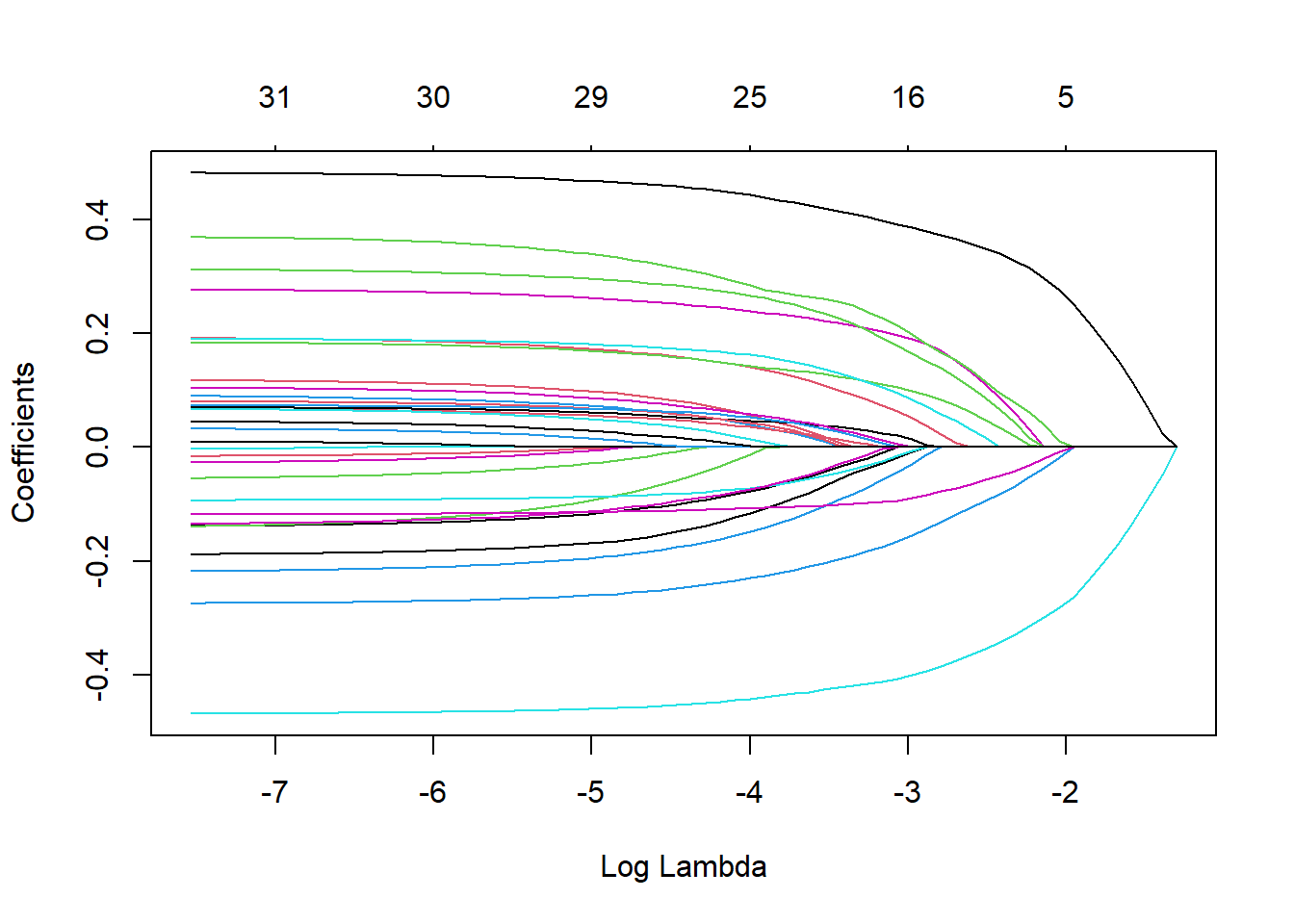

#the larger the regularization penalty, the fewer the predictors in the model

#find predictions and intervals
lasso_resid <- best_lasso_fit %>%
                  broom.mixed::augment(new_data = train_data) %>%
                  dplyr::select(.pred, BodyTemp) %>%
                  dplyr::mutate(.resid = .pred - BodyTemp)

#plot model predictions from tuned model versus actual outcomes
#geom_abline plots a 45 degree line along which the results should fall
ggplot2::ggplot(lasso_resid, aes(x = .pred, y = BodyTemp)) +
  geom_abline(slope = 1, intercept = 0, color = "red", lty = 2) +
  geom_point() +
  xlim(97, 104) + 
  ylim(97, 104) +
  labs(title = "LASSO fit: Predicted vs. Actual Body Temperature",
        x = "Actual Body Temperature (F)",
        y = "Predicted Body Temperature (F)")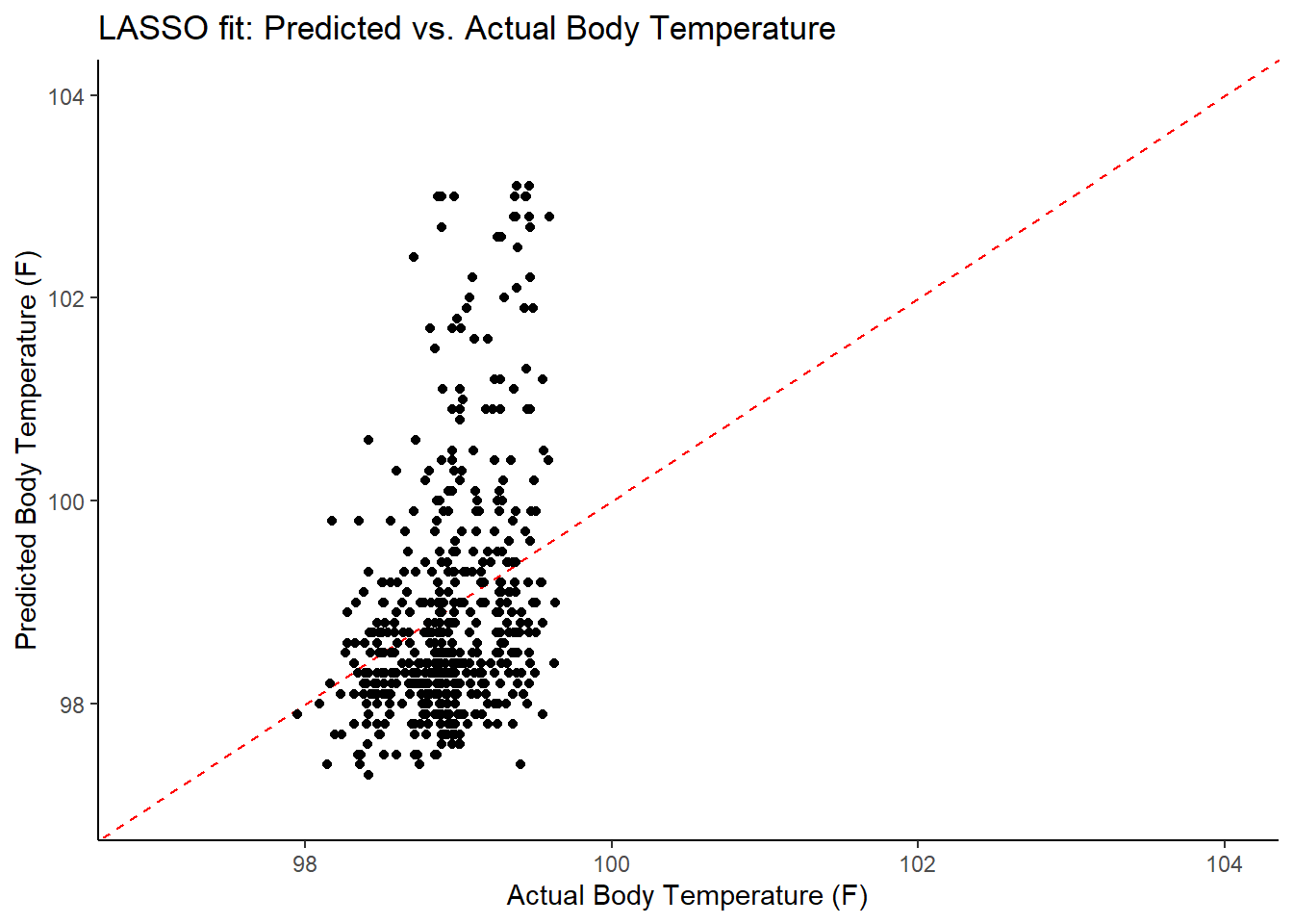

#plot model with residuals
#the geom_hline plots a straight horizontal line along which the results should fall
ggplot2::ggplot(lasso_resid, aes(x = as.numeric(row.names(lasso_resid)), y = .resid))+
  geom_hline(yintercept = 0, color = "red", lty = 2) +
  geom_point() +
  labs(title = "LASSO Fit: Residuals",
        x = "Observation Number",
        y = "Residual")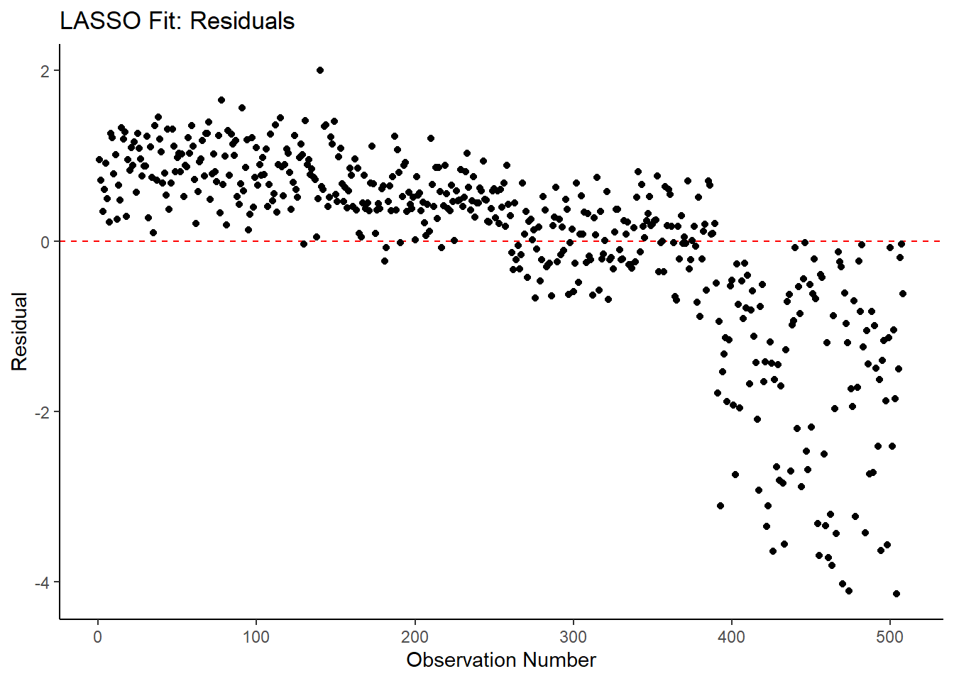

#plot model fit vs residuals
#the geom_hline plots a straight horizontal line along which the results fall
ggplot2::ggplot(lasso_resid, aes(x = .pred, y = .resid))+
  geom_hline(yintercept = 0, color = "red", lty = 2) +
  geom_point() +
  xlim(97, 104) +
  labs(title = "LASSO Fit: Residuals vs Fitted Body Temperature",
        x = "Fitted Body Temperature (F)",
        y = "Residual")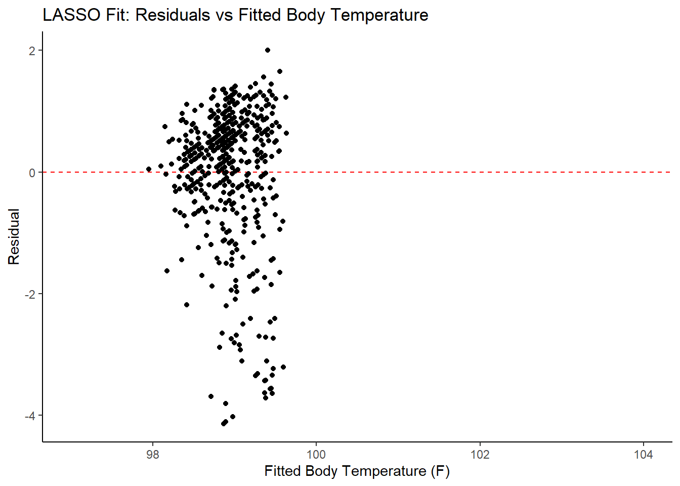

#print the 10 best performing hyperparameter sets
lasso_res %>%
  tune::show_best(n = 10) %>%
  dplyr::select(rmse = mean, std_err, penalty) %>%
  dplyr::mutate(rmse = round(rmse, 3),
                std_err = round(std_err, 4),
                `log penalty` = round(log(penalty), 3),
                .keep = "unused")

## # A tibble: 10 x 3
##     rmse std_err `log penalty`
##    <dbl>   <dbl>         <dbl>
##  1  1.15  0.0169         -2.86
##  2  1.15  0.0169         -3.10
##  3  1.15  0.017          -2.62
##  4  1.16  0.0169         -3.34
##  5  1.16  0.0169         -3.57
##  6  1.16  0.0172         -2.38
##  7  1.16  0.0168         -3.81
##  8  1.16  0.0167         -4.05
##  9  1.16  0.0175         -2.14
## 10  1.16  0.0167         -4.29

#print best model performance
lasso_performance <- lasso_res %>% tune::show_best(n = 1)
lasso_performance

## # A tibble: 1 x 7
##   penalty .metric .estimator  mean     n std_err .config              
##     <dbl> <chr>   <chr>      <dbl> <int>   <dbl> <chr>                
## 1  0.0574 rmse    standard    1.15    25  0.0169 Preprocessor1_Model18

#compare model performance to null model and tree model
lasso_RMSE <- lasso_res %>%
                tune::show_best(n = 1) %>%
                dplyr::transmute(
                  rmse = round(mean, 3),
                  SE = round(std_err, 4),
                  model = "LASSO") %>%
               dplyr::bind_rows(tree_RMSE)
lasso_RMSE

## # A tibble: 3 x 3
##    rmse     SE model       
##   <dbl>  <dbl> <chr>       
## 1  1.15 0.0169 LASSO       
## 2  1.19 0.0181 Tree        
## 3  1.21 0      Null - Train

In examining the results of the model, there is an improvement of the target metric (RMSE) under the LASSO model. However, the residual plots and observed vs fitted plots suggest the fit still isn’t ideal. Time to try one last model!

Random Forest Model

Most of the code for this section comes from the TidyModels Tutorial Case Study.

1. Model Specification

#run parallels to determine number of cores
cores <- parallel::detectCores() - 1
cores

## [1] 19

cl <- makeCluster(cores)

registerDoParallel(cl)

#define the RF model
RF_mod <-
  parsnip::rand_forest(mtry = tune(),
                       min_n = tune(),
                       trees = tune()) %>%
  parsnip::set_engine("ranger",
                      importance = "permutation") %>%
  parsnip::set_mode("regression")

#use the recipe specified earlier (line 133)

#check to make sure identified parameters will be tuned
RF_mod %>% tune::parameters()

## Collection of 3 parameters for tuning
## 
##  identifier  type    object
##        mtry  mtry nparam[?]
##       trees trees nparam[+]
##       min_n min_n nparam[+]
## 
## Model parameters needing finalization:
##    # Randomly Selected Predictors ('mtry')
## 
## See `?dials::finalize` or `?dials::update.parameters` for more information.

2. Workflow Definition

#define workflow for RF regression
RF_wflow <- workflows::workflow() %>%
               workflows::add_model(RF_mod) %>%
               workflows::add_recipe(flu_rec)

3. Tuning Grid Specification

#tuning grid specification
RF_grid <- expand.grid(mtry = c(3, 4, 5, 6),
                       min_n = c(40, 50, 60),
                       trees = c(500,1000))

4. Tuning Using Cross-Validation and the `tune_grid()` function

#tune the model with previously specified cross-validation and RMSE as target metric
RF_res <- RF_wflow %>%
              tune::tune_grid(resamples = folds,
                              grid = RF_grid,
                              control = control_grid(verbose = TRUE, save_pred = TRUE),
                              metrics = metric_set(rmse))

#look at top 5 RF models
top_RF_models <- RF_res %>%
                    tune::show_best("rmse", n = 5)
top_RF_models

## # A tibble: 5 x 9
##    mtry trees min_n .metric .estimator  mean     n std_err .config              
##   <dbl> <dbl> <dbl> <chr>   <chr>      <dbl> <int>   <dbl> <chr>                
## 1     6  1000    60 rmse    standard    1.16    25  0.0168 Preprocessor1_Model24
## 2     6   500    60 rmse    standard    1.16    25  0.0170 Preprocessor1_Model12
## 3     6  1000    50 rmse    standard    1.16    25  0.0167 Preprocessor1_Model20
## 4     5  1000    60 rmse    standard    1.16    25  0.0168 Preprocessor1_Model23
## 5     5   500    60 rmse    standard    1.16    25  0.0166 Preprocessor1_Model11

#default visualization
RF_res %>% autoplot()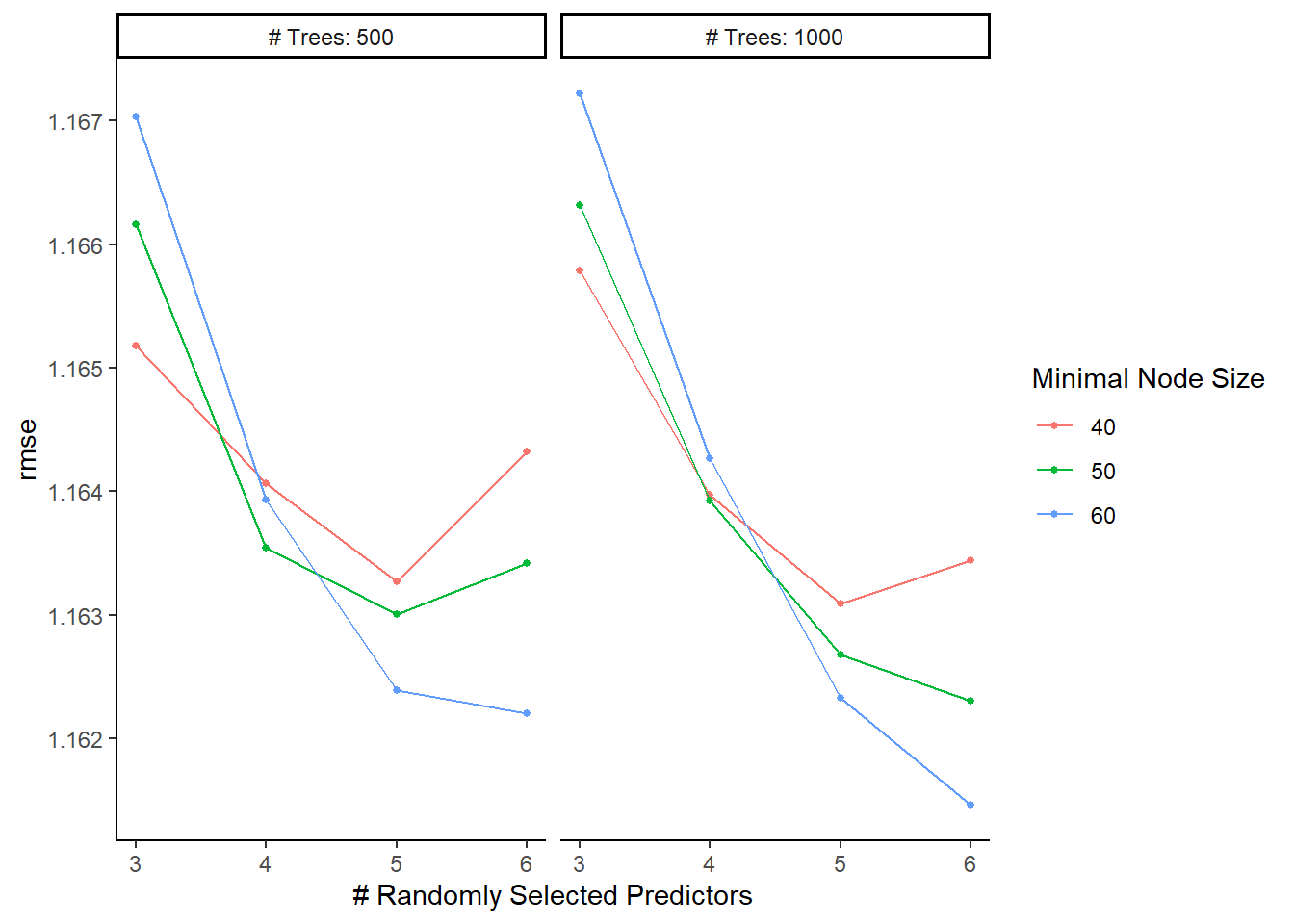

#in future analyses, might be worth more tuning with a higher minimum node size

5. Identify Best Model

#select the RF model with the lowest rmse
RF_lowest_rmse <- RF_res %>%
                      tune::select_best("rmse")

#finalize the workflow by using the selected RF model
best_RF_wflow <- RF_wflow %>%
                      tune::finalize_workflow(RF_lowest_rmse)
best_RF_wflow

## == Workflow ====================================================================
## Preprocessor: Recipe
## Model: rand_forest()
## 
## -- Preprocessor ----------------------------------------------------------------
## 1 Recipe Step
## 
## * step_dummy()
## 
## -- Model -----------------------------------------------------------------------
## Random Forest Model Specification (regression)
## 
## Main Arguments:
##   mtry = 6
##   trees = 1000
##   min_n = 60
## 
## Engine-Specific Arguments:
##   importance = permutation
## 
## Computational engine: ranger

#one last fit on the training data
best_RF_fit <- best_RF_wflow %>%
                    parsnip::fit(data = train_data)

6. Model evaluation

#extract model from final fit
x_RF <- best_RF_fit$fit$fit$fit

#plot most important predictors in the model
vip::vip(x_RF, num_features = 20)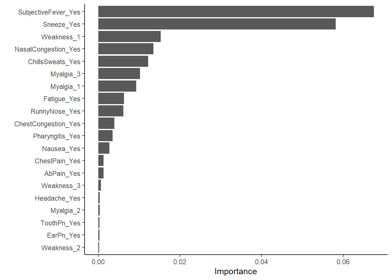

#makes sense subjective fever is the most important variable in predicting actual fever

#find predictions and intervals
RF_resid <- best_RF_fit %>%
                broom.mixed::augment(new_data = train_data) %>%
                dplyr::select(.pred, BodyTemp) %>%
                dplyr::mutate(.resid = .pred - BodyTemp)

#plot model predictions from tuned model versus actual outcomes
#geom_abline is a 45 degree line, along which the results should fall
ggplot2::ggplot(RF_resid, aes(x = .pred, y = BodyTemp)) +
  geom_abline(slope = 1, intercept = 0, color = "red", lty = 2) +
  geom_point() +
  xlim(97, 104) +
  ylim(97, 104) +
  labs(title = "RF Fit: Actual vs. Predicted Body Temperature",
        x = "Predicted Body Temperature (F)",
        y = "Actual Body Temperature (F)")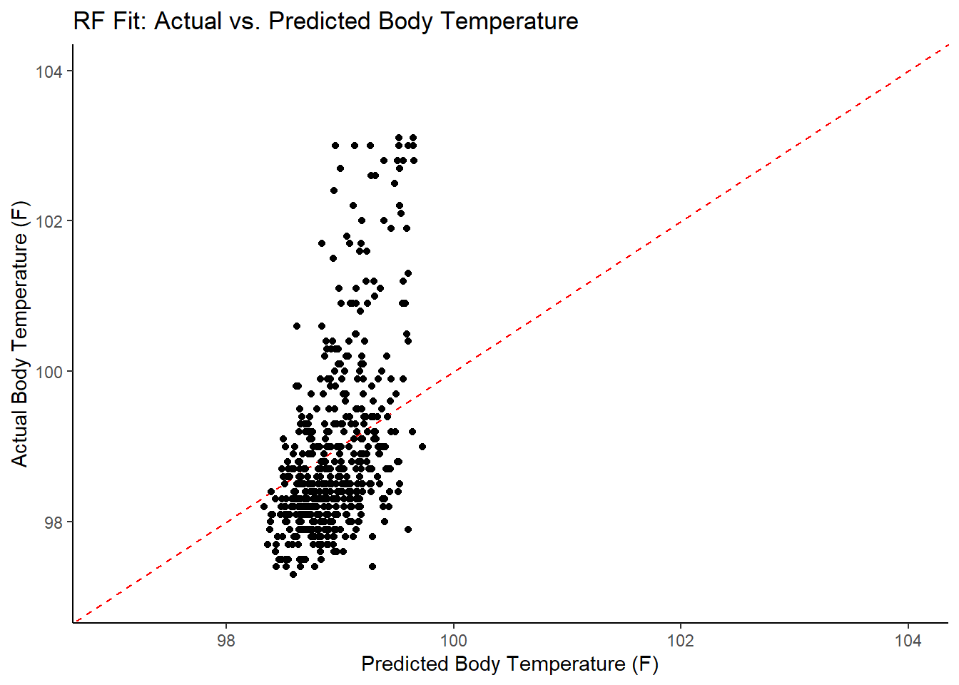

#plot model with residuals
#the geom_hline plots a straight horizontal line along which the results should fall
ggplot2::ggplot(RF_resid, aes(x = as.numeric(row.names(RF_resid)), y = .resid))+
  geom_hline(yintercept = 0, color = "red", lty = 2) +
  geom_point() +
  labs(title = "RF Fit: Residuals",
        x = "Observation Number",
        y = "Residual")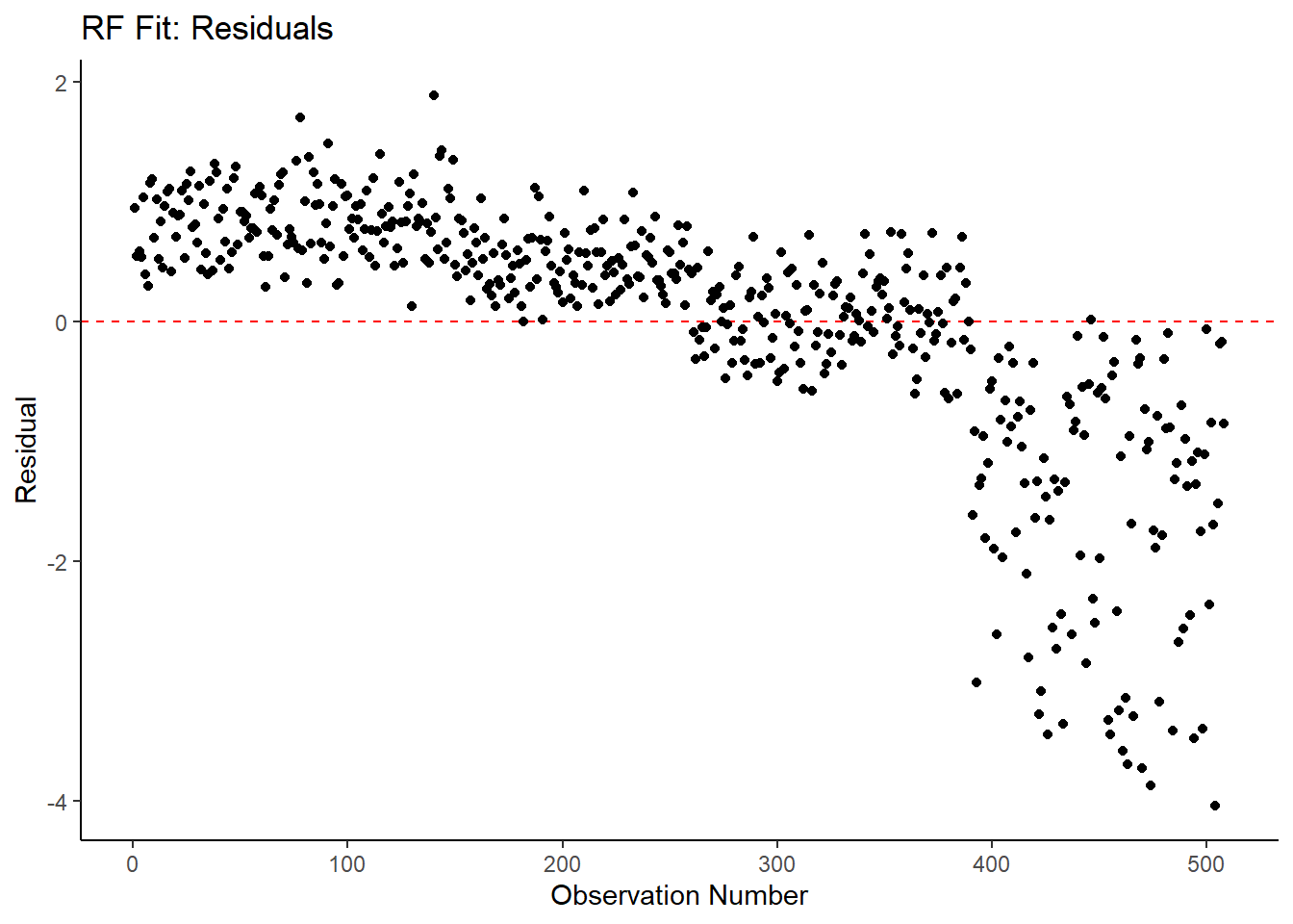

#plot model fit vs residuals
#the geom_hline plots a straight horizontal line along which the results fall
ggplot2::ggplot(RF_resid, aes(x = .pred, y = .resid))+
  geom_hline(yintercept = 0, color = "red", lty = 2) +
  geom_point() +
  xlim(97, 104) +
  labs(title = "LASSO Fit: Residuals vs Fitted Body Temperature",
        x = "Fitted Body Temperature (F)",
        y = "Residual")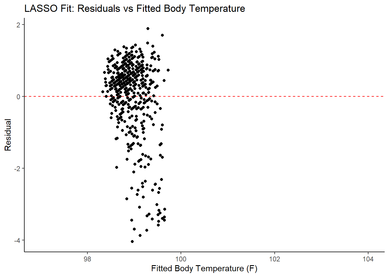

#print the 10 best performing hyperparameter sets
RF_res %>%
  tune::show_best(n = 10) %>%
  dplyr::select(rmse = mean, std_err) %>%
  dplyr::mutate(rmse = round(rmse, 3),
                std_err = round(std_err, 4),
                .keep = "unused")

## # A tibble: 10 x 2
##     rmse std_err
##    <dbl>   <dbl>
##  1  1.16  0.0168
##  2  1.16  0.017 
##  3  1.16  0.0167
##  4  1.16  0.0168
##  5  1.16  0.0166
##  6  1.16  0.0167
##  7  1.16  0.0169
##  8  1.16  0.0166
##  9  1.16  0.0167
## 10  1.16  0.0166

#print the best model
RF_performance <- RF_res %>% tune::show_best(n = 1)
RF_performance

## # A tibble: 1 x 9
##    mtry trees min_n .metric .estimator  mean     n std_err .config              
##   <dbl> <dbl> <dbl> <chr>   <chr>      <dbl> <int>   <dbl> <chr>                
## 1     6  1000    60 rmse    standard    1.16    25  0.0168 Preprocessor1_Model24

#compare model performance to null model (and other models)
RF_RMSE <- RF_res %>%
              tune::show_best(n = 1) %>%
              dplyr::transmute(
                rmse = round(mean, 3),
                SE = round(std_err, 4),
                model = "RF") %>%
             dplyr::bind_rows(lasso_RMSE)
RF_RMSE

## # A tibble: 4 x 3
##    rmse     SE model       
##   <dbl>  <dbl> <chr>       
## 1  1.16 0.0168 RF          
## 2  1.15 0.0169 LASSO       
## 3  1.19 0.0181 Tree        
## 4  1.21 0      Null - Train

In examining the results of the RF model within the context of RMSE, it does not perform better than the LASSO model. It is slightly better than the decision tree and null model.

Model Selection and Evaluation

Based on the RMSE output above, the LASSO model has the lowest RMSE and therefore is the most appropriate model in this case. The RF and Tree models are virtually identical in their performance, but all three models are an improvement over the null model. It is worth noting that none of these models actually fit the data well - suggesting the predictor variables included in this dataset aren’t all that useful in predicting the desired outcome (e.g. body temperature in suspected flu patients).

#fit lasso model to training set but evaluate on the test data
lasso_fit_test <- best_lasso_wflow %>%
                    tune::last_fit(split = data_split)

#compare test performance against training performance
lasso_rmse_test <- collect_metrics(lasso_fit_test) %>%
  dplyr::select(rmse = .estimate) %>%
  dplyr::mutate(data = "test")

lasso_comp <- lasso_RMSE %>%
                  dplyr::filter(model == "LASSO") %>%
                  dplyr::transmute(rmse, data = "train") %>%
                  dplyr::bind_rows(lasso_rmse_test) %>%
                  dplyr::slice(-3) #don't know why the third row shows up
lasso_comp

## # A tibble: 2 x 2
##    rmse data 
##   <dbl> <chr>
## 1  1.15 train
## 2  1.15 test

#RMSEs are essentially identical --> what we want (suggests we might've avoided overfitting)

#find predictions and intervals
lasso_resid_fit <- lasso_fit_test %>%
                  broom.mixed::augment() %>%
                  dplyr::select(.pred, BodyTemp) %>%
                  dplyr::mutate(.resid = .pred - BodyTemp)

#plot model predictions from tuned model versus actual outcomes
#geom_hline plots a 45 degree line, along which the results should fall
ggplot2::ggplot(lasso_resid_fit, aes(x = .pred, y = BodyTemp)) +
  geom_abline(slope = 1, intercept = 0, color = "red", lty = 2) +
  geom_point() +
  xlim(97, 104) +
  ylim(97, 104) +
  labs(title = "LASSO fit: Predicted vs. Actual Body Temperature",
        x = "Predicted Body Temperature (F)",
        y = "Actual Body Temperature (F)")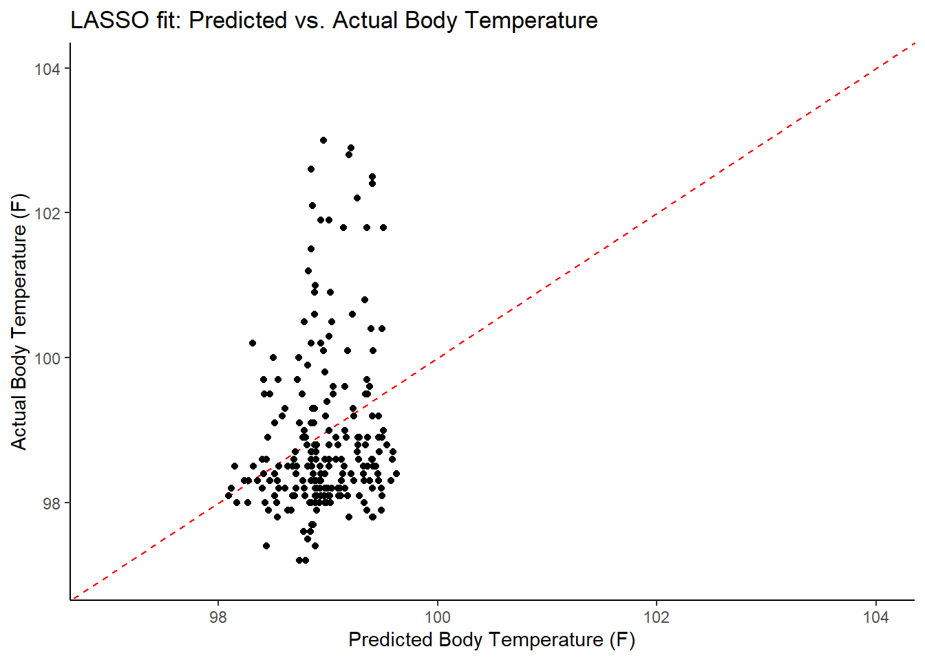

#plot model with residuals
#the geom_hline plots a straight horizontal line along which the results should fall
ggplot2::ggplot(lasso_resid_fit, aes(x = as.numeric(row.names(lasso_resid_fit)), y = .resid))+
  geom_hline(yintercept = 0, color = "red", lty = 2) +
  geom_point() +
  labs(title = "Lasso Test Fit: Residuals",
        x = "Observation Number",
        y = "Residual")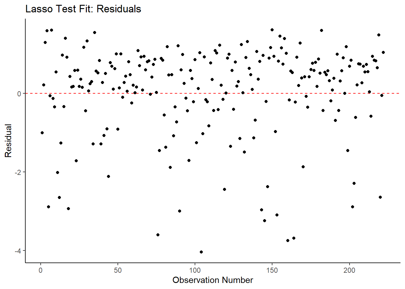

#plot model fit vs residuals
#the geom_hline plots a straight horizontal line along which the results fall
ggplot2::ggplot(lasso_resid_fit, aes(x = .pred, y = .resid))+
  geom_hline(yintercept = 0, color = "red", lty = 2) +
  geom_point() +
  xlim(97, 104) +
  labs(title = "LASSO Test Fit: Residuals vs Fitted Body Temperature",
        x = "Fitted Body Temperature (F)",
        y = "Residual")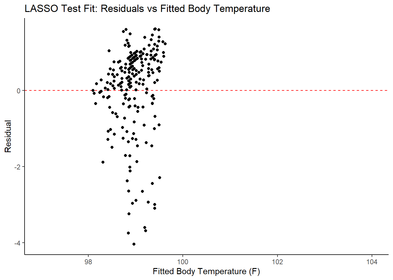

Overall Conclusion

None of the models used in this analysis predict the chosen outcome (actual body temperature) all that well. There’s a variety of potential reasons for this - all of which warrant further consideration in an actual research project. Most notably, not every patient with influenza will have a fever. It would be interesting to repeat this analysis with other outcomes with which influenza typically present (e.g. cough, sore throat, myalgia, etc.).

Influenza Project - Machine Learning Models

Introduction

Required Packages

Load Data

Data Setup

Null model performance

Tree Model

1. Model Specification

2. Workflow Definition

3. Tuning Grid Specification

4. Tuning Using Cross-Validation and the tune_grid() function

5. Identify Best Model

6. Model evaluation

LASSO Model

1. Model Specification

2. Workflow Definition

3. Tuning Grid Specification

4. Tuning Using Cross-Validation and the tune_grid() function

5. Identify Best Model

6. Model evaluation

Random Forest Model

1. Model Specification

2. Workflow Definition

3. Tuning Grid Specification

4. Tuning Using Cross-Validation and the tune_grid() function

5. Identify Best Model

6. Model evaluation

Model Selection and Evaluation

Overall Conclusion

4. Tuning Using Cross-Validation and the `tune_grid()` function

4. Tuning Using Cross-Validation and the `tune_grid()` function

4. Tuning Using Cross-Validation and the `tune_grid()` function